FlowMol
Most of this text is converted from the latex version of my Thesis (available here). As a result, many of the link to other sections will not work, so it is advised to view the thesis for more details. As of 2021, this code is available as Open-Source on Github. It comes with minimal documentation and no guarentee of validity as it is my person research code, but if someone want to use it, I am very happy to discuss collaborations.
1 Introduction
This section outlines the development, verification, profiling and functionality of the molecular dynamics (MD), continuum computational fluid dynamics (CFD) and coupler codes (CPL) developed or utilised during this project. The main purpose of this section is to support the results obtained in later sections by verifying the accuracy of the code against peer-reviewed publications, experiments and analytical solutions. This section also aims to serve as an introduction to each of the codes for future users as well as a series of tests which the user can recreate to verify new developments. The CPL library, developed in section 4 of this page, is a novel contribution of this work. It should be a useful tool for researchers allowing them to coupled their own high performance CFD and MD schemes and retain the scaling of both.
This page is organised as follows, the first section 2, contains an introduction to the new molecular dynamics solver developed as part of this project. A major component of the work completed has been the development of a new high-fidelity MD code, written using state-of-the-art optimisation techniques and developed to run in parallel using the Message Passing Interface (MPI) paradigm. A description of the numerical scheme is presented in subsection 2.1, the force optimisations in subsection 2.2 and code features are outlined in subsection 2.3. The optimisations, parallelisation, and profiling are discussed in subsection 2.4. Finally, a full range of verification tests are presented in section 2.5.
In section 3, the Continuum Fluid Dynamics (CFD) solvers used during this project are discussed. The first subsection 3.1 introduces a new simple finite volume CFD solver developed for the purpose of testing the coupling schemes. The code’s features and its verification are briefly described. A brief description of the features of this code and the important changes required for coupling are outlined.
The final part of this page, section 4 outlines the key features of the coupler library (CPL). The verification and implementation of this code is also included. The CPL library is a novel contribution, and is available as open source software (Smith & Trevelyan, 2013).
2 Molecular Dynamics Solver
2.1 Numerical Scheme
Molecular dynamics requires the solution of Newton’s laws for an N-body system. Under the assumption of classical, non-relativistic system, the evolution of the molecules is described exactly by Newton’s laws,
mi iγ iγ = Fiγ = Fiγ | (1) |
ṙiγ = ṙiγ = ṙiγ + +   iγ iγ + +  ... r
iγ ... r
iγ + O(Δt3) + O(Δt3) | (2) | |
ṙiγ = ṙiγ = ṙiγ − −  iγ iγ + +  ... r
iγ ... r
iγ + O(Δt3). + O(Δt3). | (3) |
 iγ iγ Δt = ṙiγ Δt = ṙiγ −ṙiγ −ṙiγ . . | (4) |
miṙiγ = miṙiγ = miṙiγ + ΔtFiγ + ΔtFiγ . . | (5) |
 and the velocity at t− 1∕2Δt allows the velocity
at t + 1∕2Δt to be obtained. A similar process is applied to obtain the position at
the next time step t + Δt,
and the velocity at t− 1∕2Δt allows the velocity
at t + 1∕2Δt to be obtained. A similar process is applied to obtain the position at
the next time step t + Δt,
ṙiα = =  ![[riα (t+ Δt )− riα (t)]](MD_coding27x.png) | (6) |
riα = riα = riα + ṙiα + ṙiα Δt Δt | (7) |
Any numerical approximation of an integral is normally judged for its
truncation error - how well it represents the integral. The Verlet leap frog
algorithm is a central difference formulation and the truncation error is of order
four  (4) due to the cancelling of the third order terms. In addition to this good
order of accuracy, it can be shown that the Verlet algorithm is symplectic (phase
space conserving). As a result, it displays excellent total energy (Hamiltonian)
conservation (Rapaport, 2004). This is due to the central nature of the numerical
scheme where any error is damped rather than allowed to build up over
time.
(4) due to the cancelling of the third order terms. In addition to this good
order of accuracy, it can be shown that the Verlet algorithm is symplectic (phase
space conserving). As a result, it displays excellent total energy (Hamiltonian)
conservation (Rapaport, 2004). This is due to the central nature of the numerical
scheme where any error is damped rather than allowed to build up over
time.
It is also possible to use an iterative scheme to integrate the equations of motion, the velocity Verlet, which has also been developed as part of the project.
2.2 Force calculation
The interaction potential between the molecules is the only approximation in the process and, for the work in this section, it is described by the Lennard-Jones potential,
Φ(|rij|) = 4ϵ![[( ) ( ) ]
-ℓ- 12 -ℓ- 6
rij − rij](MD_coding31x.png) ,|rij|≤|rc|, ,|rij|≤|rc|, | (8) |
In its simplest form, computation of pairwise molecular interactions requires N2 calculations for a system of N molecules. The required N interaction calculations for a given molecule are shown in Figure (1a). As the Lennard-Jones potential drops off rapidly with distance, the majority of the N2 calculations are negligible. Enforcing a cutoff distance, rc, over which the potential is not evaluated allows the calculation to be significantly accelerated, as only local interactions need to be computed. A commonly used cutoff length is |rc| = 21∕6, known as the Week-Chandler-Anderson (WCA) potential (Rapaport, 2004). This sets the cutoff length to the minimum of the potential well, removing the attractive tail. This has the advantage that the cutoff is short, resulting in far fewer interaction calculations and significantly faster simulations. This potential is useful for representative simulation, however a cutoff of |rc| > 2.5 is typically required to correctly model many physical process. The use of a cutoff rc allows the N2 inter-molecular calculations to be reduced to order N. This is achieved by splitting the domain into a series of cutoff length sized cells and considering only the interactions between molecules in neighbouring cells. This reduces the task of checking all pairs of interactions to just a local check over the molecules in the current and adjacent cells. The list of molecules per cell can be built efficiently using integer division. The division into cells is shown in Figure (1b) where the grey circle represents molecules within cut off radius rc and the current and adjacent cells can be seen to form a cube that contains all interacting molecules.
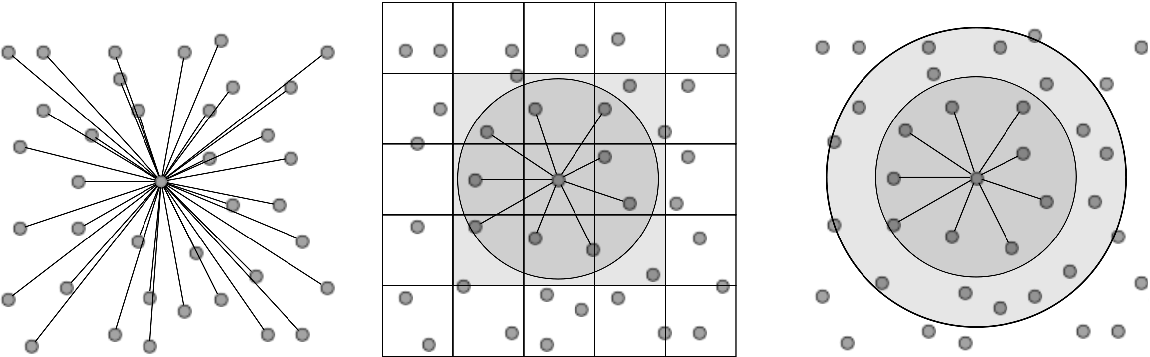
Further improvements are obtained by keeping a list of only the interacting neighbours to a given molecule. This ensures calculation of the forces on a molecule requires only the checking of molecules in the surrounding sphere instead of the surrounding cube of adjacent cells. Building the neighbour list, however, is more expensive than the cell list as it requires conditional checking based on a sphere local to each molecule. To optimise this, the cell list is used to construct the neighbour list, but with larger cells. The resulting sphere containing neighbour molecules has a radius larger than |rc|, as shown in Figure (1c), so that rebuilding is not required every timestep. This extra distance can then be tuned for each case (using parameter studies) to optimise the checking sphere size (e.g. rc + 0.3) and rebuild frequency (e.g. 15). Further improvement in efficiency is made using Newton’s third law to halve the number of interactions calculated. For further details of these methods see for example Rapaport (2004).
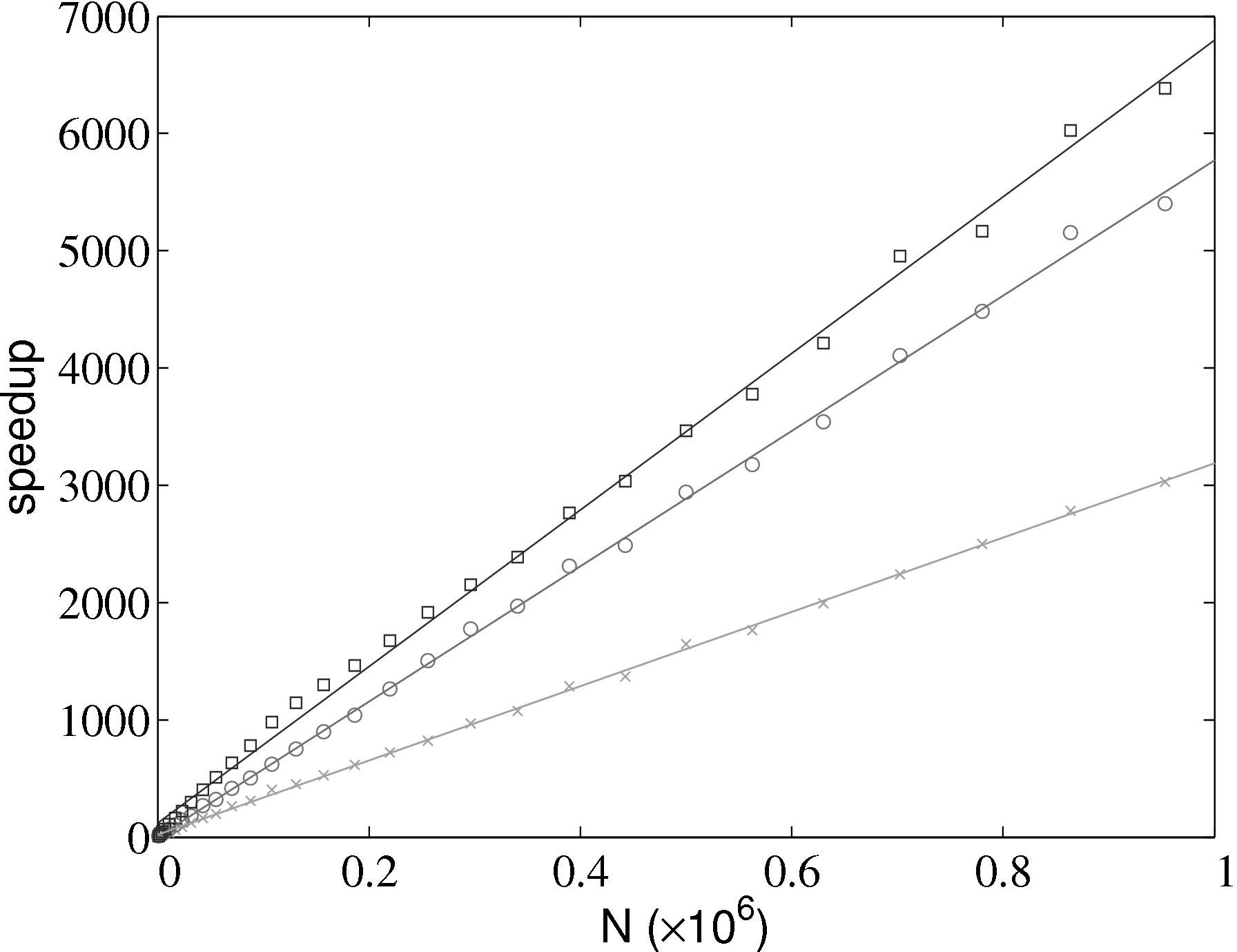
The improvement in simulation efficiency for the molecular dynamics solver has been tested up to a system size of one million molecules, shown in Figure 2. The time taken for a given simulation case, tcase, is divided by the time for the all pairs case, tap, in order to obtain a speedup metric. These improvements result in a simulation which now scales as N.
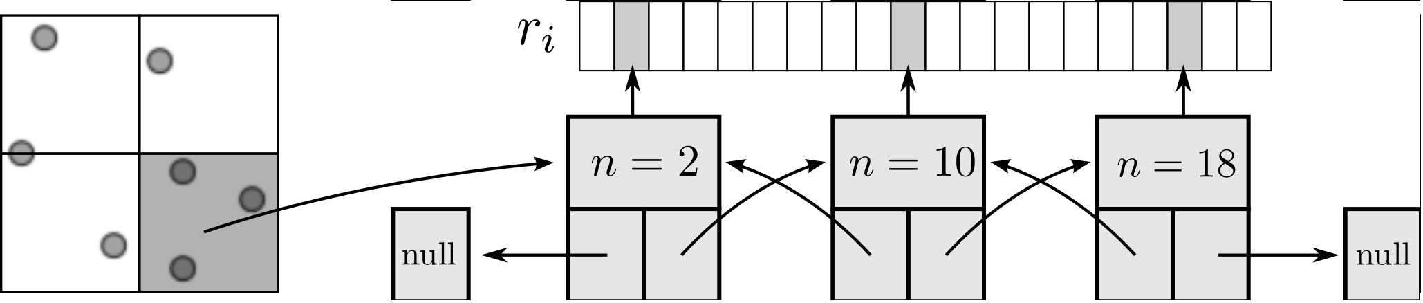
As the size of the cell/neighbour lists are not known in advance, an arbitrary array would need to be allocated to contain all possible interactions. This array would grow or develop gaps as the essential interactions change and molecules move in and out of range. To avoid this problem, a linked lists system is used. Linked lists are a chain of FORTRAN data types connected by pointers (see Figure 3). Each data type has an integer with the interacting molecule number n and the pointer to the next (and previous) data type in the list. The molecular number n identifies the location in memory of the molecule. This can be used to load the molecules position ri, velocity ṙi, acceleration ai, etc. The top and the bottom item in a list point to the null pointer which identifies the end of the linked list. Each linked list is associated with a given cell (or molecule in the neighbour list case). An array of head types contains the number of items in each list and a pointer to the head element.
All cell or neighbour list operations are performed by a library of subroutines developed to build, manipulate and destroy linked lists. This function library includes linklist print, search, pop and push routines which prevent the user from having to deal with the list pointers directly. These routines have been fully tested for memory leaks with Valgrind (Nethercote, 2004) and ‘soak tested’ for a wide range of different cases.
2.3 Code details
This subsection contains details of the code structure, philosophy and key features.
2.3.1 Code Structure
The code is structured in a modular way. The source code files are grouped into four types: setup files (setup*), simulation files(simulation*), finalisation files (finish*) and general library files (e.g. modules.f90, linklist.f90, messenger.f90). Each group performs the following tasks:
- Setup - Routines to initialise a new simulation or read in an old restart file; parameters are set by the free form keyword based input file; arrays are allocated, the messenger processor topology is initialised and output files are opened.
- Simulation - Routines which advances the code by calculating molecular interactive forces and advancing the molecular trajectories. A spatial decomposition is used for parallelism and message passing is used to exchange halos between the processes. Outputs are written at user specified intervals.
- Finish - Save final state files, finish and close outputs and deallocate all arrays
- General library files - Routines used throughout the setup, simulation and final parts of the code. All MPI routines are called through a messenger file which has a parallel and serial version. Linklists manipulation and other general library routines are included in this category
Compilation is performed using a makefile in the code directory. The code has been tested on a number of compilers (Intel FORTRAN, gfortran, cray, gnu, pgi) and architectures (HECToR, Imperial’s CX1/2, Linux Red Hat/Ubuntu, Apple Mac OS and Windows). The makefile uses compiler information from a range of verified cases on various architectures built up during the code’s development and is designed to be easily supplemented when porting to new platforms. The serial code is self-contained with no links to external libraries and the parallel code requires only access to the MPI modules. There are a range of build options including serial and parallel versions along with a number of debug, profiling and optimisation options.
The code reads a freeform keyword based input file which entirely specifies the simulation parameters and required outputs and analysis. Most keywords are optional and a default value is used if the keyword is missing. There is also a restart facility which reads in the parameters, molecular positions and velocities from a previous simulation. The restart file is written in the same format in serial or parallel using the MPI2 I/O libraries. The spatial position of a molecule and its storage location in memory are not always consistent. As a result, restarts on different processor topologies require re-ordering. This is performed on start-up for small systems (procs < 33). For large system, parallel re-ordering is an inefficient use of time on a supercomputer – therefore a separate serial code to reorder is provided.
2.3.2 Features Overview
Some of the features developed for the molecular dynamics code include,
Flow control | Molecular | Output |
Gaussian Thermostat | Momentum/Energy/ |
|
Tethered Atoms (Petravic & Harrowell, 2006) | VMD visualisation (Humphrey et al., 1996) |
|
Constrained Dynamics ((O’Connell & Thompson, 1995; Nie et al., 2004; Flekkoy et al., 2000)) | Solid/Liquid | Stress Tensor |
SLLOD algorithm (Evans & Morriss, 2007) | Sliding/moving walls | Radial Distribution Function |
2.3.3 Version Control and collaborative code development
A fully verified and working code is hosted on a subversion server to allow simultaneous development by multiple users. To prevent corruption of the codes core functionality, a number of bash and python scripts are used to check serial/parallel restarts along with other benchmarks. These are run periodically to help in pinpointing errors introduced by code developments. The MD code has been extended by other users to include more thermostats, integration algorithms, Lees Edwards sliding boundaries and the suite of tools needed to simulate a range of polymers.
2.4 Computational Developments
This subsection contains a description of the serial and parallel developments, optimisations and benchmarking results for the MD solver.
2.4.1 Profiling and optimising the serial code
The interaction lists detailed in section 2.2 are the single biggest improvement to the computational speedup of the MD solver. However, a number of other improvements are possible as outlined in this section. The code is compiled with full optimisation flags and profiled using gprof (and later Tau) to obtain a detailed breakdown of time spent on various operations. This profiling data is compared to established MD codes (DL_POLY and LAMMPS). This process is used to identify routines which take longer than established codes – these then become the focus for optimisation. All profiling for the MD solver, DL_POLY and LAMMPS is performed on one core of the same quad core desktop (IntelⓇ Core (TM) 2 Quad CPU Q9300 @ 2.50GHz with 4GB of RAM).
Optimisation is separated into two types: limiting required operations and memory access optimisations.
- Operations limiting improvements include limiting branching statements inside loops, re-using calculated data by defining intermediate variables, moving operations out of loops (as far as possible) and forcing function in-lining using compiler directives.
- Memory access optimisations include minimising memory allocations, avoiding superfluous temporary array creations and maximising cache efficiency. As moving through linked list results in non-contiguous data access and reduced cache efficiency, the code is checked using Valgrind’s cachegrind. The cache misses are minimised by changing nested loop order and sorting data in memory. In order to sort the data to maximise cache hits, the positions of the molecules in memory are reordered based on spatial locality. A recursive function to generate 3D Hilbert curves provides the ordering in memory of the molecules. This is thought to provide the best mapping of the 3D spatial locality of molecular positions to 1D memory (Anderson et al., 2008). There is a substantial reduction in cache misses after re-ordering and a noticeable increase in speed of simulation for large system sizes and longer simulations.
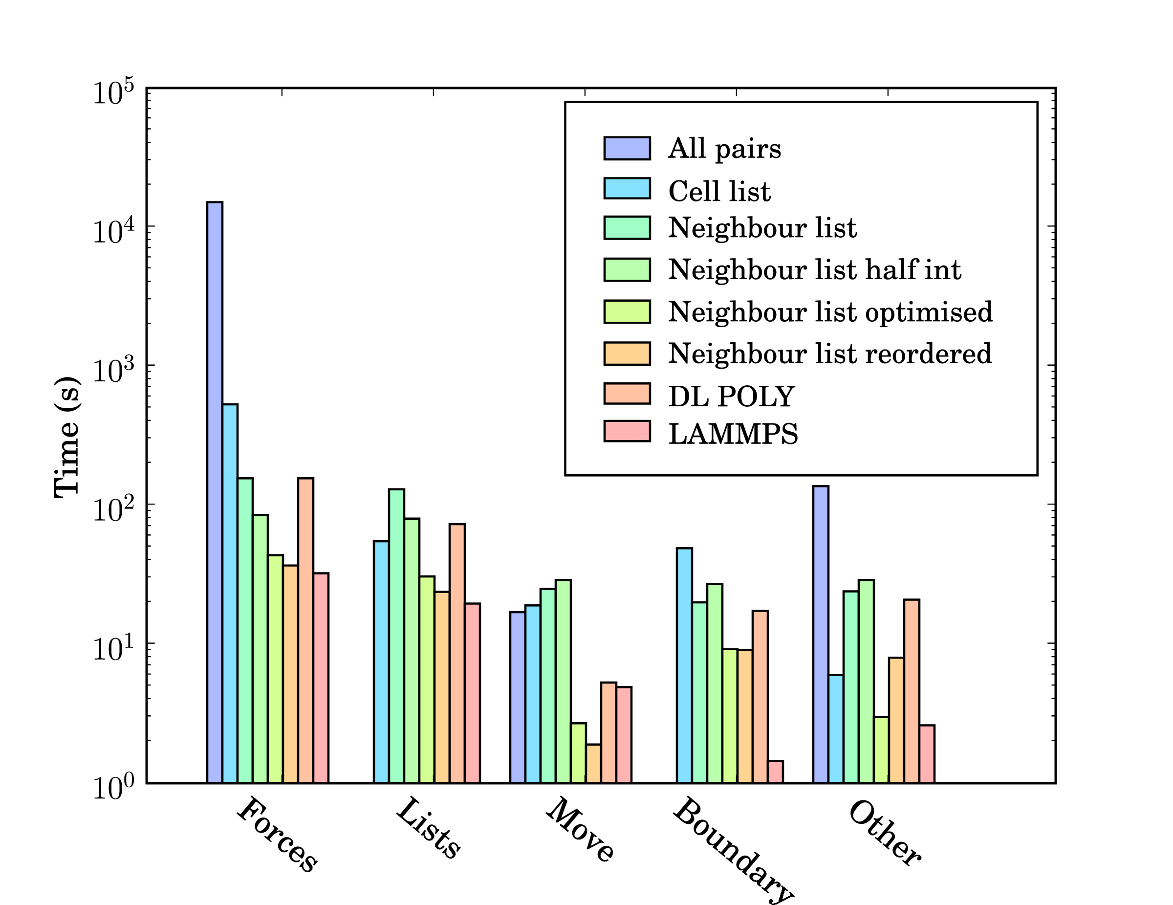
In addition, profile-guided optimisation is used to tune the compilation of the executable based on profiling data gathered from representative simulations. The results of these successive optimisations are summarised by chart 5 together with a comparison to LAMMPS (svn revision 8808) and DL_POLY (version 4.03). The required operations for a molecular dynamics simulation can be divided into five main areas; force calculation (forces), cell/neighbour list building and manipulation (lists), movement of the molecules (move), exchange of boundary information using halos (boundary) and other operations (other) including collecting statistics, re-ordering data and compiler internal operations such as memory manipulations (e.g. __intel_new_memset is often in the top five most expensive routines).
The force routine is the most expensive part of the calculation and the successive improvement attempts focus on this. Moving from all pairs to cell lists represents the biggest change with over an order of magnitude improvement. The cell to neighbour list improvements, detailed in section 2.2, have the disadvantage of requiring greater list building time – although this is offset by the improvements in force computation. The next three optimisations include using Newton’s 3rd law to halve the number of interactions calculated (neighbour list half int), using aggressive compiler based optimisation flags with other optimising operations outlined above (Neighbour list optimised), and finally memory based optimisation and sorting (Neighbour list reordered). The sorting can be seen to improve the speed of the forces,lists, move and boundary routines by more than the increased time taken to sort (included in other).
DL_POLY is a FORTRAN based code while LAMMPS is written in C++. The performance of LAMMPS can be seen to be significantly better than DL_POLY and so it is taken as the benchmark. In total, LAMMPS can be seen to be faster than the MD solverby a factor of 1.3. Profiling data indicates that the force calculation take a similar amount of time in LAMMPS and the MD solverwith re-ordering (which LAMMPS also employs). Manipulation of the interaction list, including neighbour and cell list building is slower in the MD solver. This may be, in part, a consequence of using linked lists in FORTRAN – these dynamic data structures are not native to FORTRAN and require significant manipulation to build and search. They would also likely be missed by FORTRAN compiler optimisation heuristics. The movement of molecules is faster in the MD solveras the leap frog algorithm is used (instead of the velocity Verlet used by LAMMPS, requiring twice the number of calculations per timestep).
The performance gap of 1.3 between LAMMPS and the in-house written MD code is deemed acceptable. LAMMPS has existed since the mid-1990s and has been the subject of extensive optimisation and development by Sandia labs, Lawrence Livermore National labs, at least three companies and many researchers and computer scientists. The performance difference may be a result of the comparisons between C++ and FORTRAN codes, especially using gprof, which was developed for C++. This is supported by a disproportionate amount of the time spent in routines which appear to be internal to the compiler (other). In addition, the performance of the MD solverrelative to the FORTRAN code DL_POLY is extremely favourable.
2.4.2 Parallel computation of MD simulation using the Message Passing Interface (MPI)(Gropp et al., 1999a)
Three different methods have been employed to parallelise molecular dynamics simulations on distributed computing hardware. The first is based on atomic decomposition in order to distribute the molecules evenly between processors. The second is to divide the most computationally intensive step, the force calculation, over the different processors with each taking a section of the calculation. The final decomposition method subdivides the domain into individual regions, with each processor responsible for the integration of atomic trajectories in an assigned region.
Each of these methods has advantages under certain conditions. For example, an atomic decomposition provides natural load balancing, but requires large amounts of data passing for all but the smallest system. Plimpton’s (Plimpton, 1995) analysis of the different methods concludes that, for short range systems with large numbers of molecules, a spatial decomposition scheme provides the best performance. Most commonly used parallel MD codes make use of spatial decomposition, including GROMACS (Spoel et al., 2005), DL_POLY and LAMMPS (Plimpton et al., 2003), as well as the algorithm used in this work. This approach also matches the parallel model employed for the continuum solver, which is beneficial for the purpose of algorithmic interfacing.
Verification of the parallel algorithm is performed by comparing the results for the same case in serial and parallel: a simulation started in serial saves an initial state, which is then read by the serial and parallel versions of the program (where the atoms are distributed to processor by their location in parallel). This ensures identical starting configurations.
The intermolecular force calculation in parallel requires each processor to exchange information with adjacent processors at each timestep (halo-exchange). Molecules must also be passed between processors when they leave the processor domain, a process which only occurs every rebuild time for neighbour-list calculations. The process of gathering statistics requires accumulation of data on a single root processor, as well as MPI operations that govern data writing by individual processors to a shared file, using the MPI2 standard (Gropp et al., 1999b).
The details of a typical communication run are addressed in the next section through profiling data which is used to optimise parallel performance of the code.
2.4.3 Profiling and optimising the parallel code
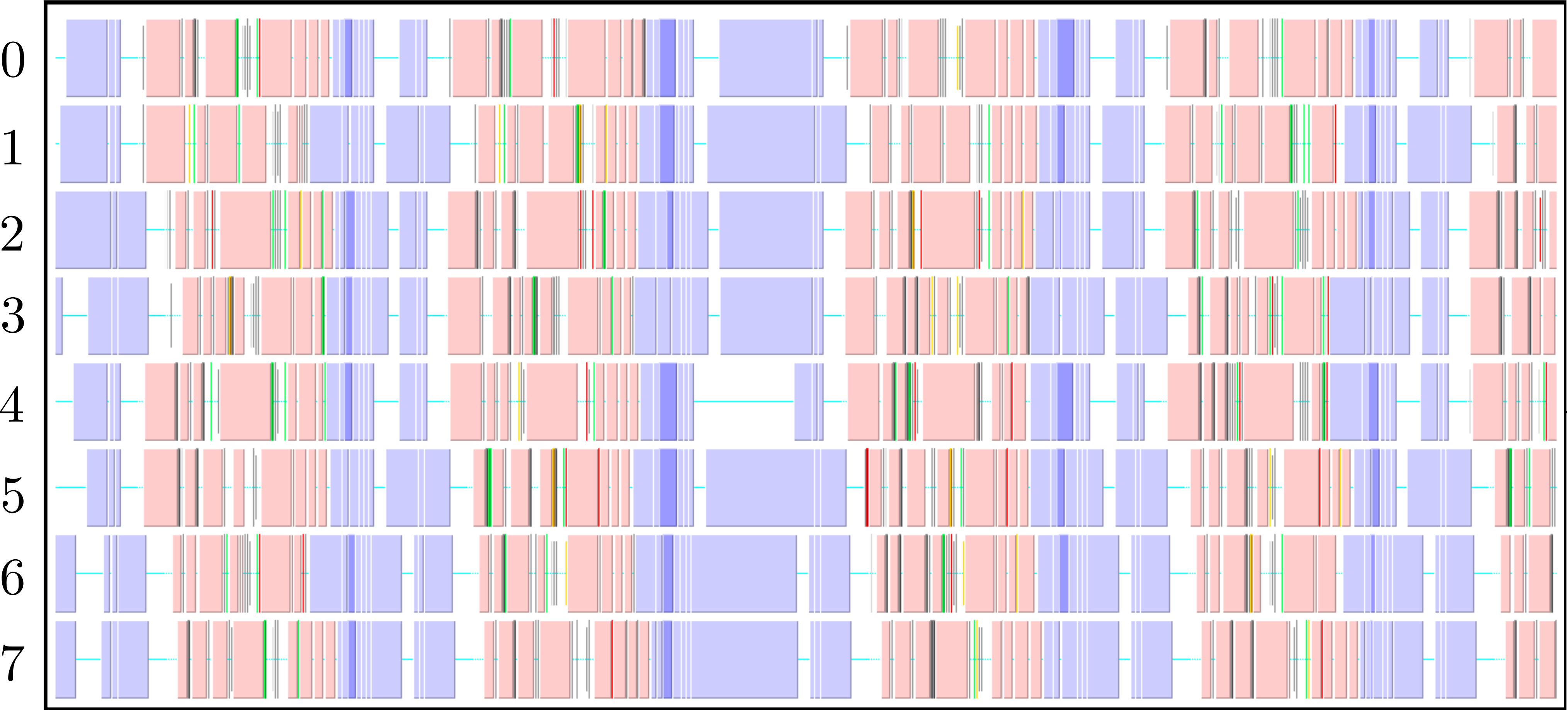
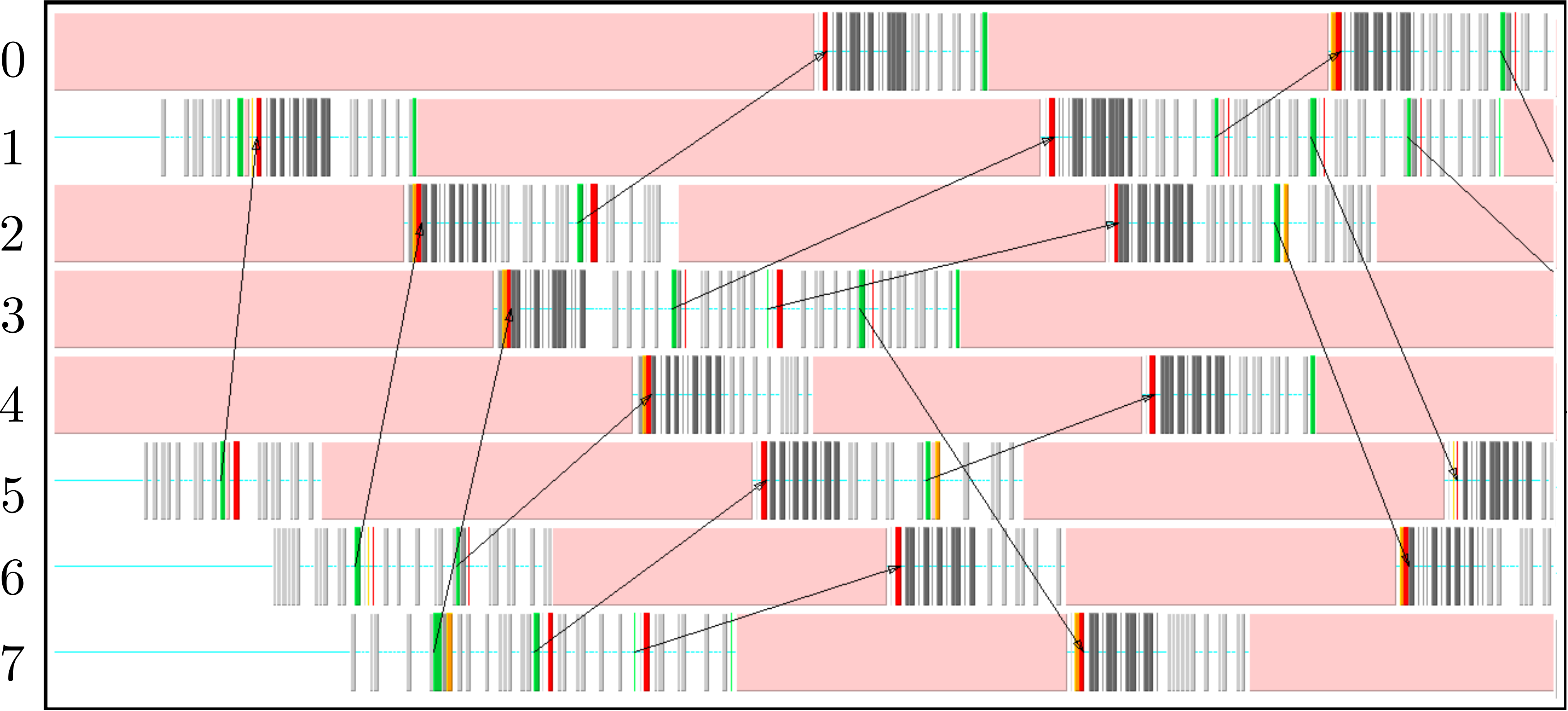
The parallel code is profiled using MultiProcessing Environment (mpe) libraries which trace the communication patterns during an MD simulation. An example of this logging data is included in Figure 6, giving an insight into the parallel MD solver. The simulation is performed using eight processors (2 × 2 × 2) solving a periodic WCA fluid using the neighbour lists. MPI communications on the eight processors are shown on the vertical axis against time on the horizontal. Figure 6a shows an overview of approximately 3 simulation timesteps, split into alternating sections of blue and red/yellow/green blocks. The blue blocks are global (blocking between all processors) and take far more time than the many local exchanges represented by the collection of red/yellow/green blocks. Figure 6b shows further details of these local exchanges.
The communication process starts by packing the data into buffers to send (light grey blocks). As the number of molecules a processor will receive is not known a-priori, the receiving processors use MPI_probe (light red blocks) to establish how much data they expect to receive before allocating appropriate memory. The MPI_send command (green) is posted on a given processor where the black arrows on Figure 6b trace the movement of a message to the corresponding MPI_receive (dark red) command on another processor. The receives are non-blocking, so a MPI_wait command (orange) is placed before the received data is required. The new molecular data is unpacked using MPI_unpack (dark grey blocks). The neighbour-list must be rebuilt when a molecule has moved sufficient distance. As a local rebuild necessitates a global rebuild, rebuild checks must be broadcast to ensure the neighbour-list is up to date. The blue blocks in Figure 6a are global communications (gather/scatter) to check for this rebuild (together with exchange of other information required for rebuilding).
 (a) Overview of a rebuild interval
 (b) Detailed view of data exchange
The profiling above is useful as it identifies areas to improve performance. MPI_probe is clearly inefficient and should be replaced by the sending of arbitrary sized buffers followed by a check for overflow. In addition, gather/reduce operations should be limited, for example by disabling the global rebuild check (usually satisfied every 15 steps) for an initial periods of time (e.g. first 10 steps) .
A parallel performance logging tool, Tau (Shende & Malony, 2006), was also employed. This allows the user to compare time spent in computationally intensive routines, like the force calculation, to waiting times for MPI communications. As a result, optimisation can focus on expensive parallel routines and establishing the optimum particles-per-processor to balance computation and communication. Use of profiling tools periodically during developments and before submission of long jobs help to optimise the utilisation of supercomputing resources.
2.4.4 Benchmark of Parallel scalability
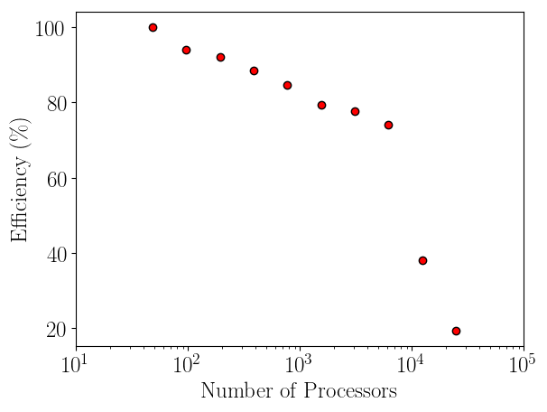
Having verified the parallel code, it can be benchmarked for parallel scalability. Weak scaling on ARCHER (2018) is shown here up to 24.6k cores,
 = tp1∕(ntpn).
The initial performance drop in using one, two, four then eight cores is attributed to the increased complexity of passing data in one, two and three dimensions respectively. In serial, the molecular data is simply copied internally. With two cores, only two faces must be passed, in two dimensions, four edges and four faces must be passed. For the eight core cases, twelve edges, six faces and eight corners must be passed separately. If scaling is instead defined vs the eight core speed, the code can be shown to be 94% efficient on 1024 processors.
2.4.5 A note on Graphical processing units (GPU)
The use of GPU acceleration was investigated as part of the development of the molecular dynamics code. General purpose GPUs have been shown to give massive increases in computational speeds. Current state of the art molecular dynamics application suggest a 30 times speed up over the same code run on a CPU (Anderson et al., 2008). NVIDIA Compute Unified Device Architecture is used as the programming model (the standard Open CL is under developed while NVIDIA have invested heavily in CUDA) (NVIDIA, 2010). CUDA is a C based set of libraries, with some C++ extensions, allowing calculations to be performed on the GPU. As the majority of the code is FORTRAN, C based wrappers are used to allow variables to be passed from FORTRAN to C++ and then to CUDA C.
The first attempt to optimise the MD solverdelegated only the force calculation to the GPU. The positions of all interacting pairs of molecules were passed to the GPU and the forces passed back. The performance improvement was found to be negligible as the time to copy the large numbers of interacting pairs negated any computational speed up.
The next attempt at optimisation involved copying a single set of molecular positions into GPU global memory and calculating the interaction forces. Although this showed some speed up, the improvements were still very limited. The exchange of data still greatly reduces any benefit in speed up. This is a similar discovery to the work Brown et al. (2011), where without neighbour list builds on the GPU, the force calculation on a GPU was actually found to be slower (0.7 speedup). In order to gain the 30 times speed up, the entire code (forces, movement, list building and averaging) would need to be ported to the GPU with data exchange only for i/o (Anderson et al., 2008). For a serial GPU this represents an entire redesign of the MD solverfor the GPU architecture, with all future developments written to maintain this structure.
The aim of this project is to model very large coupled runs, often simulating more molecules than a single GPU could store. This would require multiple CPUs (connected by MPI) linking together the multiple GPUs (ideally with clever use of page locked memory) (NVIDIA, 2010). Load balancing would also be required in order to ensure the available resources are efficiently utilised (Brown et al., 2011). Even with load balancing and multiple CPUs linked to multiple GPUs, speed up of only 2.5 are reported when the force calculations (rc = 2.5) alone performed on the GPUs (Brown et al., 2011). Due to the complexity of implementation, the inflexibility of development and the added complication of required coupling to CFD codes, it was decided to postpone the GPU development until CUDA libraries are sufficiently improved.
2.5 Verification
As a new molecular dynamics code has been developed, full verification is essential before use as a research tool. This section outlines a range of verification cases against standard benchmarks and experimental results. The tests include energy conservation and trajectories, radial distribution functions (RDF), phase diagrams and non-equilibrium molecular dynamics (NEMD) simulations of canonical fluid mechanical flows.
2.5.1 Energy Conservation
The first and most important tests of a molecular dynamics algorithm are those
related to conservation of momentum and energy. Total energy conservation is
actually a highly sensitive test of the correctness of a program (Allen &
Tildesley, 1987). This is the first verification test after each successive algorithm
change. The interchange between kinetic and potential energy as well as the total
energy is shown in Figure 8 for the 
 ensemble (constant number of molecules
, olume and nergy). This simulation used a WCA potential with a
truncation distance rc = 21∕6 and 2048 molecules initialised in an 8 × 8 × 8 FCC
lattice with reduced density of 0.8 and temperature of 1.0. As a result, molecules
start outside of interaction range and the initial potential energy is zero.
Periodic boundaries are used in all three directions. All quantities are
given in terms of the length ℓ, atomic interaction strength ϵ and mass
m of the particle so the LJ potential equation 8 with ℓ = ϵ = m = 1
is,
ensemble (constant number of molecules
, olume and nergy). This simulation used a WCA potential with a
truncation distance rc = 21∕6 and 2048 molecules initialised in an 8 × 8 × 8 FCC
lattice with reduced density of 0.8 and temperature of 1.0. As a result, molecules
start outside of interaction range and the initial potential energy is zero.
Periodic boundaries are used in all three directions. All quantities are
given in terms of the length ℓ, atomic interaction strength ϵ and mass
m of the particle so the LJ potential equation 8 with ℓ = ϵ = m = 1
is,
Φ(rij) = 4![[ −12 −6]
rij − rij](MD_coding41x.png) . . | (9) |
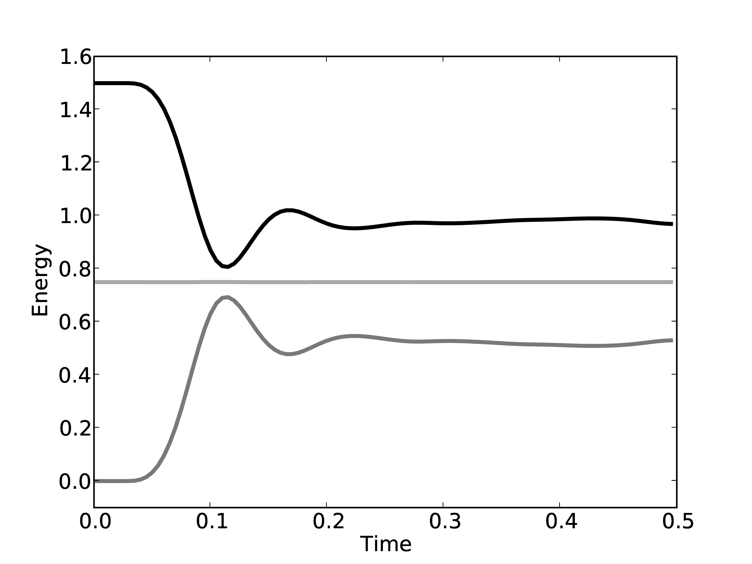
The total energy remains (almost) constant, while the kinetic and potential interchange can be seen by the mirrored peaks and troughs. The use of the leapfrog algorithm to discretise the equation of motion is known to give good long time energy conservation properties. However, it can be seen that for very long simulations some energy drift occurs. Quantitative verification is performed by matching various parameter to the book by Rapaport (2004) such as evolution of total energy.
| Rapaport Table 2.1 | This Work’s Simulation
| ||||||
| step | KE | Total
| Pressure | KE | Total
| Pressure | |
| 100 | 0.6592 | 0.9952 | 4.5371 | 0.6472 | 0.9951 | 4.6392 | |
| 200 | 0.6490 | 0.9951 | 4.5829 | 0.6442 | 0.9950 | 4.6686 | |
| 300 | 0.6397 | 0.9951 | 4.6454 | 0.6643 | 0.9951 | 4.3660 | |
| 400 | 0.6477 | 0.9951 | 4.5675 | 0.6325 | 0.9951 | 4.6938 | |
| 500 | 0.6596 | 0.9951 | 4.4702 | 0.6349 | 0.9951 | 4.6563 | |
| 1000 | 0.6480 | 0.9950 | 4.5496 | 0.6391 | 0.9950 | 4.7037 | |
| 2000 | 0.6497 | 0.9951 | 4.5371 | 0.6257 | 0.9951 | 4.7560 | |
| 3000 | 0.6539 | 0.9952 | 4.5184 | 0.6582 | 0.9952 | 4.4758 | |
| 7000 | 0.6370 | 0.9952 | 4.6203 | 0.6684 | 0.9952 | 4.3523 | |
Note that the total energy in both systems is the same from the start of the simulation and stays constant throughout the time history of the simulation. The kinetic energies however, fluctuate in different ways in the two systems as they evolve through phase space along completely different trajectories.
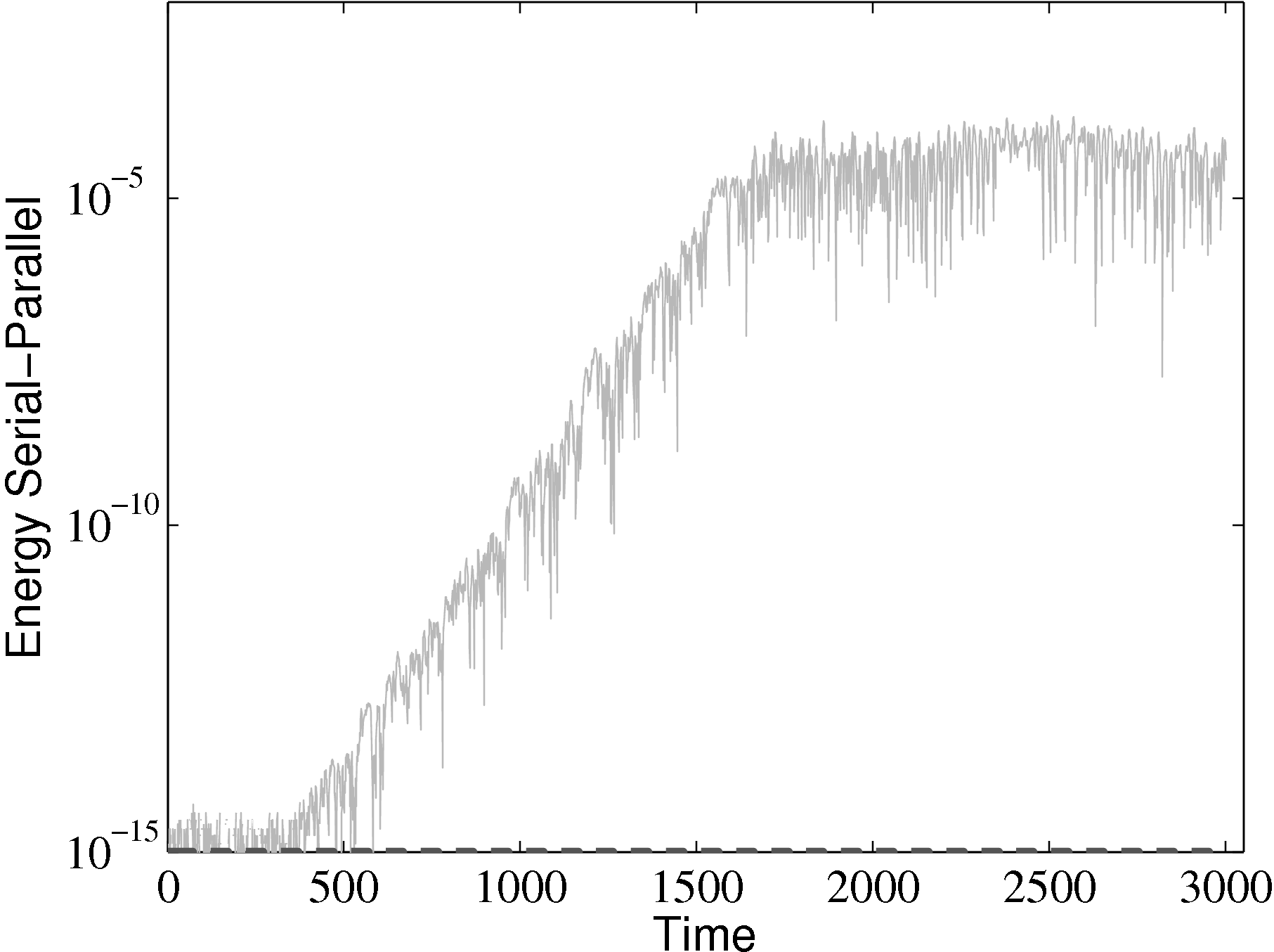
parallel
from the parallel solution minus the serial solution serial divided by the
serial solution: [parallel −serial]∕serial.
The different evolutions of kinetic energy in table 1 represents a very important phenomenon in molecular simulation, which is the chaotic behaviour. This is an inevitable consequence of employing a finite precision computer in the solution of the equations of motion. Chaotic behaviour has wide ranging implications for molecular simulation, the most immediate of which is that matching the evolution of energy, or indeed any property between two molecular systems, is impossible beyond a certain number of timesteps. To demonstrate this, two identical simulations (same input data, operations and computer architecture/compiler) were run on a single processor and then split between two processors. The comparison of these two systems (serial-parallel) is shown in Figure 9. The divergence of trajectories, although initially at the limit of precision for a single molecule, eventually grows to 0.01% after 200 reduced time units and plateaus. This is because the system’s total energy is the same (to within 0.01% flucatations) and only the initial trajectories differ. This behaviour is observed for any changes to order of operations (during code development) or comparisons between restarted calculations. For this reason, initial agreement and trajectory divergence must be taken into account during the verification of changes made to parallel/serial codes. Any verification of new code developments therefore consist of checking agreement for the initial period of time (up to the divergence at ∼ 1500 time units) and agreement of long time statistical properties.
The next table 9 compares the variation in energy at different densities to the values reported in Rapaport (2004). Very good agreement can be seen between the obtained results and those of Rapaport (2004).
| Density | Rapaport Table 2.2 | This Work’s Simulation
| ||||
| Total Energy | KE | Pressure | Total Energy | KE | Pressure | |
| 0.8 | 0.650 | 0.995 | 4.537 | 0.650 | 0.997 | 4.554 |
| 0.6 | 0.823 | 0.994 | 1.954 | 0.823 | 0.995 | 1.964 |
| 0.4 | 0.915 | 0.994 | 0.815 | 0.915 | 0.995 | 0.818 |
2.5.2 Radial Distribution Functions
Further tests of the three dimensional code included comparing the radial distribution function (RDF), g(r) as shown in Fig. 10.
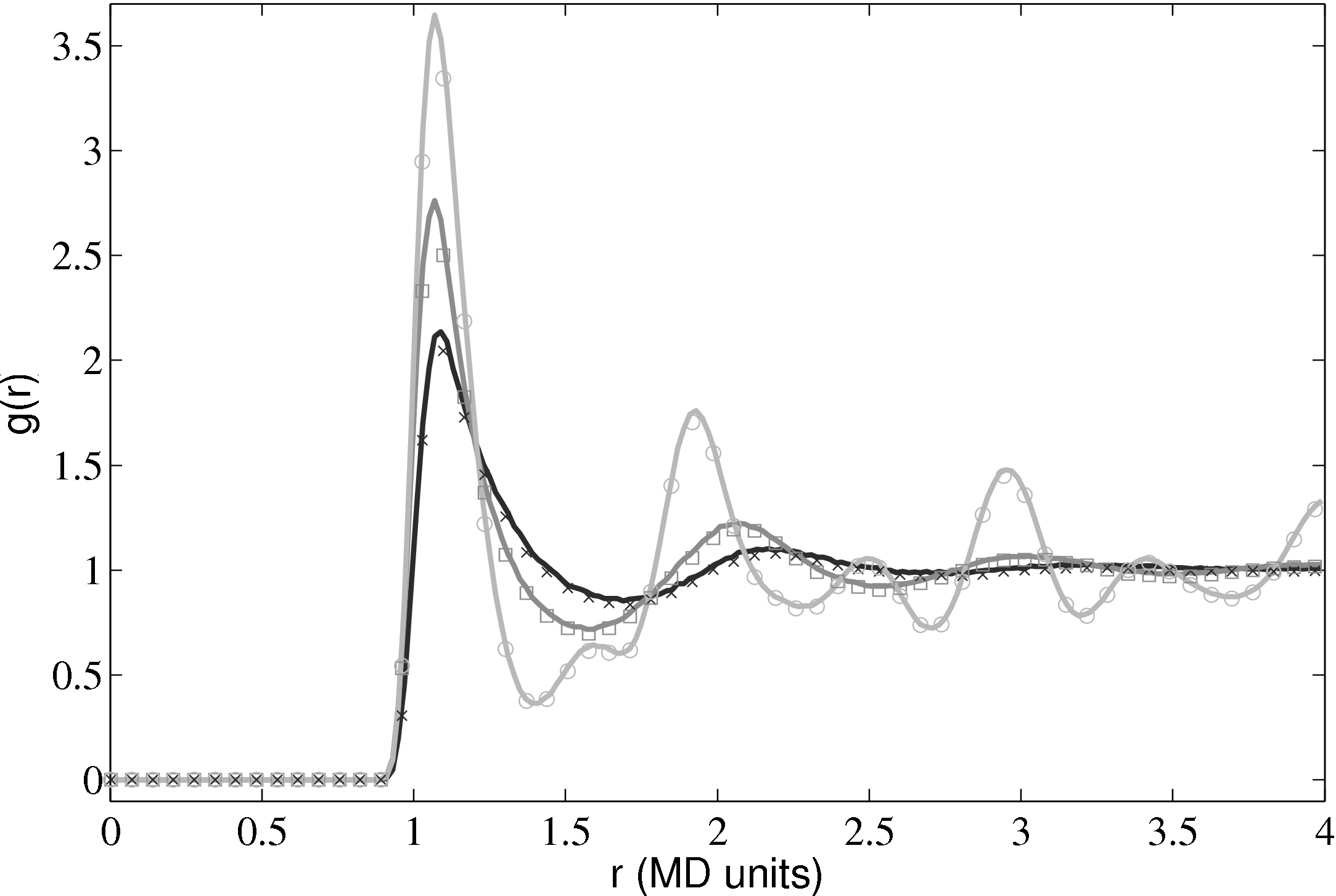
The RDF is a normalised measure of the local particle number density as a function of distance r from the centre of an arbitrary particle. Peaks and troughs indicate the presence of coordination shells and inter-shell regions, respectively. The RDF shows a key difference from models based on a dilute gas and a molecular dynamics simulation. It is for this reason that a full molecular simulation is required when small length scale effects become important.
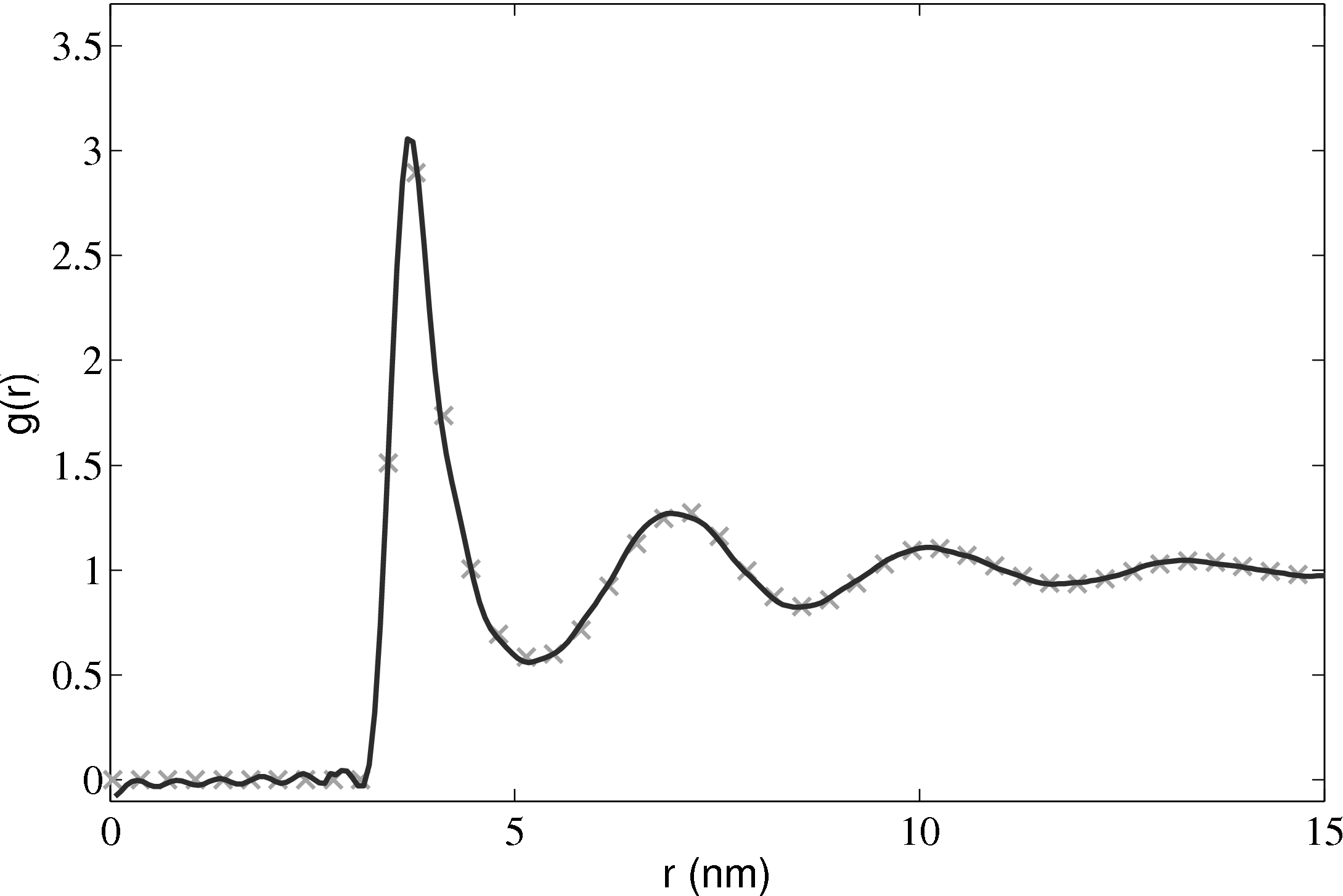
The radial distribution function is an important quantity as it can also be obtained from experiments. For liquid Argon, experimental data from Yamell et al. (1973) with T = 85K and ρ = 0.02125Å−3 is shown in Figure 11. In MD units this is T∗ = 0.708 and ρ∗ = 0.8352; simulation results for the corresponding case are shown on the same Figure 11.
2.5.3 Phase diagrams
Phase diagrams are a thorough test of a molecular model over a range of different conditions. By adjusting the density and temperature the model is tested over a range of operating conditions – from solid to gas. Phase diagrams also allow verification of features such as the Nosé-Hoover thermostats and pressure calculations. The change of phase from a liquid to a solid can be observed for the lower temperature/density cases.
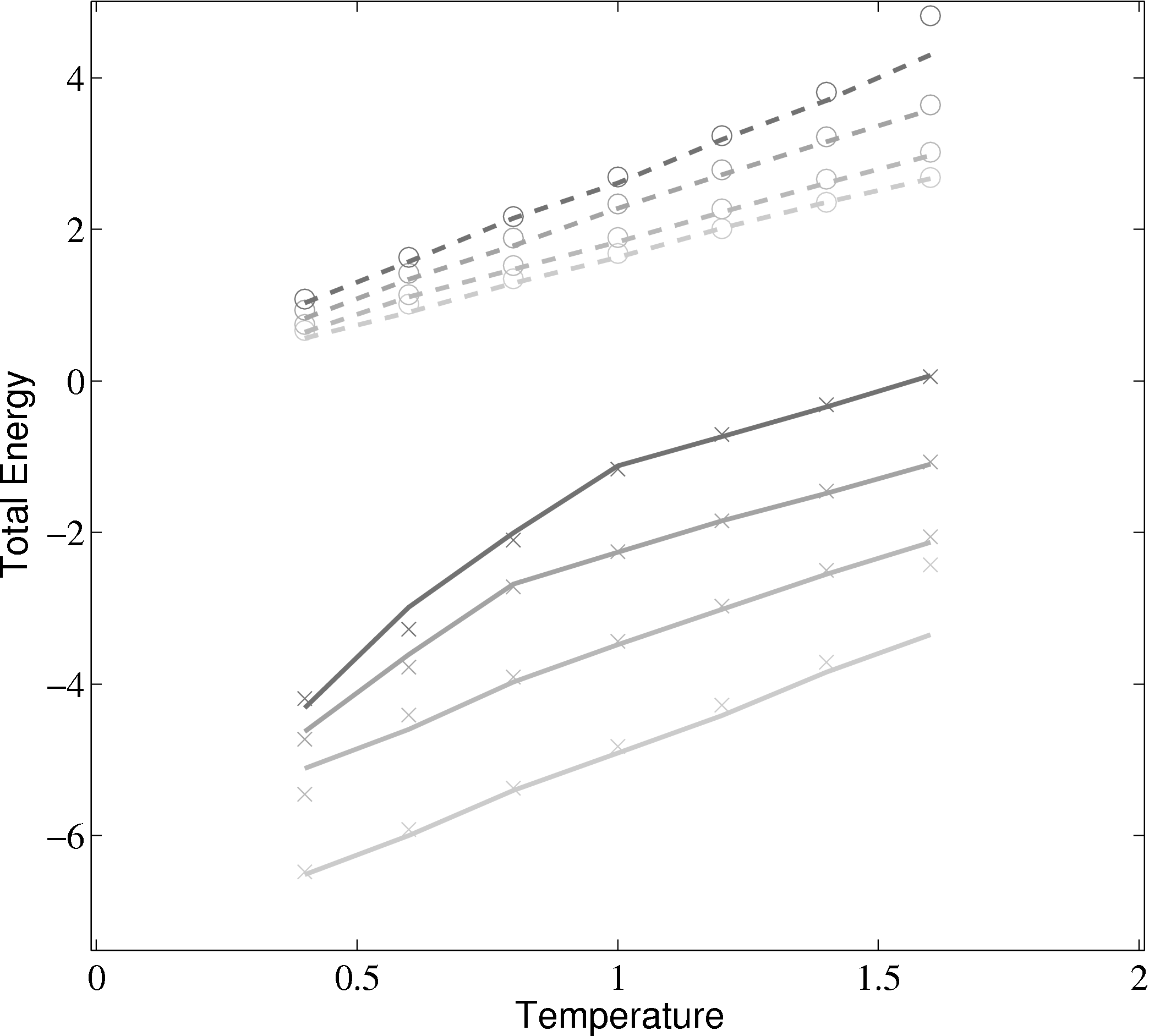 (a) Total energy vs temperature from MD code compared with
Rapaport (2004)
(a) Total energy vs temperature from MD code compared with
Rapaport (2004)
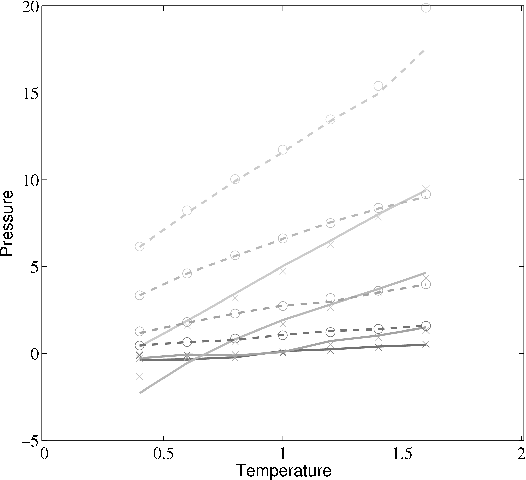 (b) Pressure vs temperature from MD code compared with
Rapaport (2004)
(b) Pressure vs temperature from MD code compared with
Rapaport (2004)
 ); (×) MD code Lennard-Jones
(rc = 2.5) (∘) MD code WCA; (■) ρ = 0.4; (■) ρ = 0.6; (■) ρ = 0.8; (■)
ρ = 1.0
); (×) MD code Lennard-Jones
(rc = 2.5) (∘) MD code WCA; (■) ρ = 0.4; (■) ρ = 0.6; (■) ρ = 0.8; (■)
ρ = 1.0
In comparing the results from the present MD code to those of Rapaport (2004), the LJ energy has been corrected using the standard long range correction factors (Allen & Tildesley, 1987) and the pressure results are not corrected. It is not clear from the text in Rapaport (2004) if this correction is applied to the energy or pressure. Rapaport (2004) suggests applying the correction to energy and not pressure as the magnitude is negligible in the latter case.
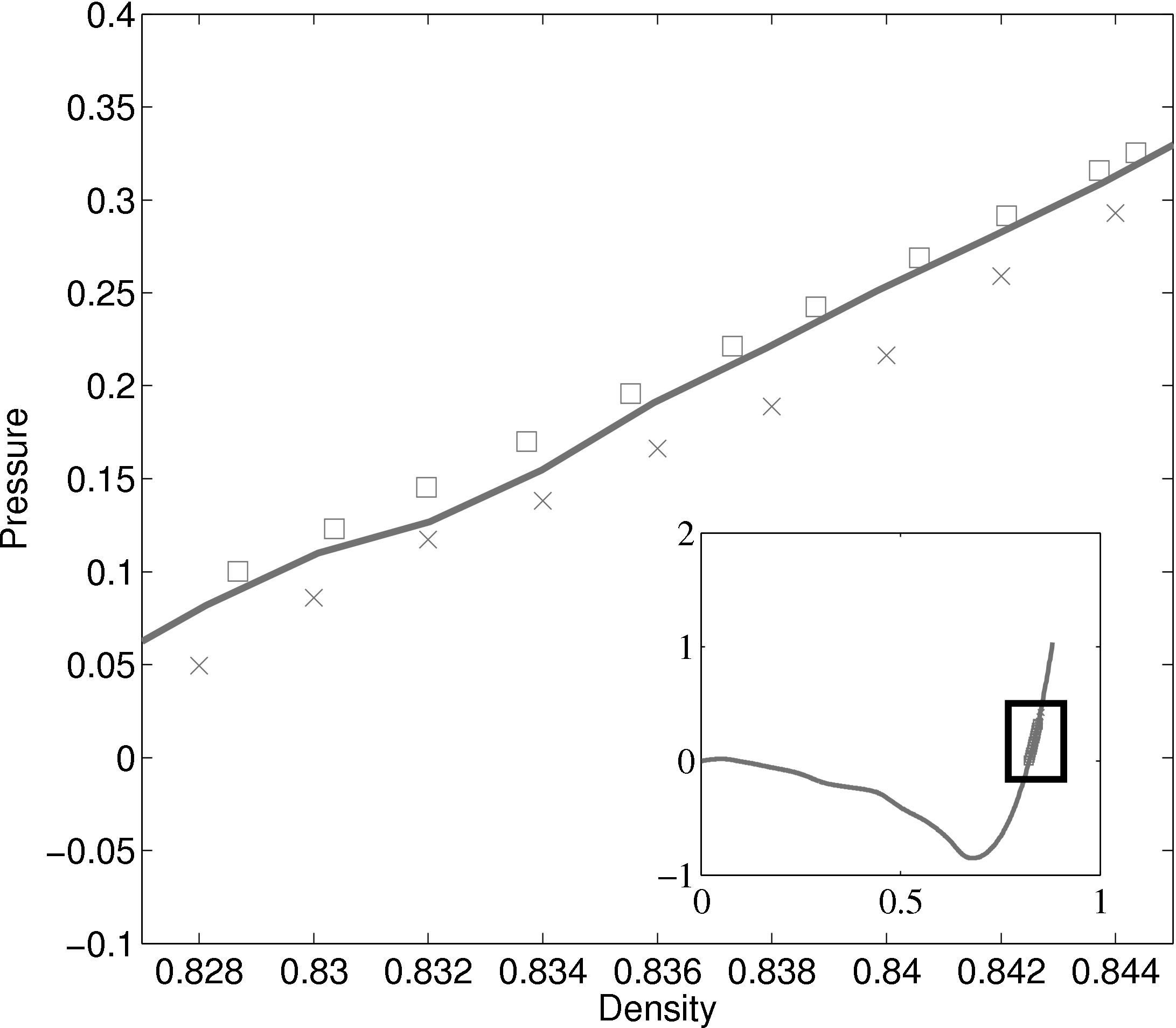
The density-pressure relationships also agree with experimental data for liquid Argon at a temperature of 90.1K (T∗ = 0.75), Itterbeek & Verbeke (1960), as well as reference data for the LJ potential calculated using grand-canonical transition-matrix Monte Carlo (GCMC) (NIST, 2013). The experimental data is only available for a small density range. The GCMC reference data for the whole range is shown on the insert. In order to match the pressure, the standard long range correction must be applied. Reasonable agreement is observed to the experimental results.
2.5.4 Non-equilibrium molecular dynamics simulations
Continuum fluid flow problems for which there exist analytical solutions to the Navier-Stokes provide a convenient test for non-equilibrium molecular dynamics (NEMD) algorithms. The case of Couette flow is considered here, using the time evolving analytical solution derived in appendix of Smith (2014) thesis,
u(y,t) = ∑
n=1M −  sin sin + U0φ + U0φ , , | (10) |
Couette Flow
In this study, Couette flow was simulated by entraining a model liquid between two solid walls. The top wall was set in translational motion parallel to the bottom (stationary) wall and the evolution of the velocity profile towards the steady-state Couette flow limit was followed. All dimensions are given in MD units.
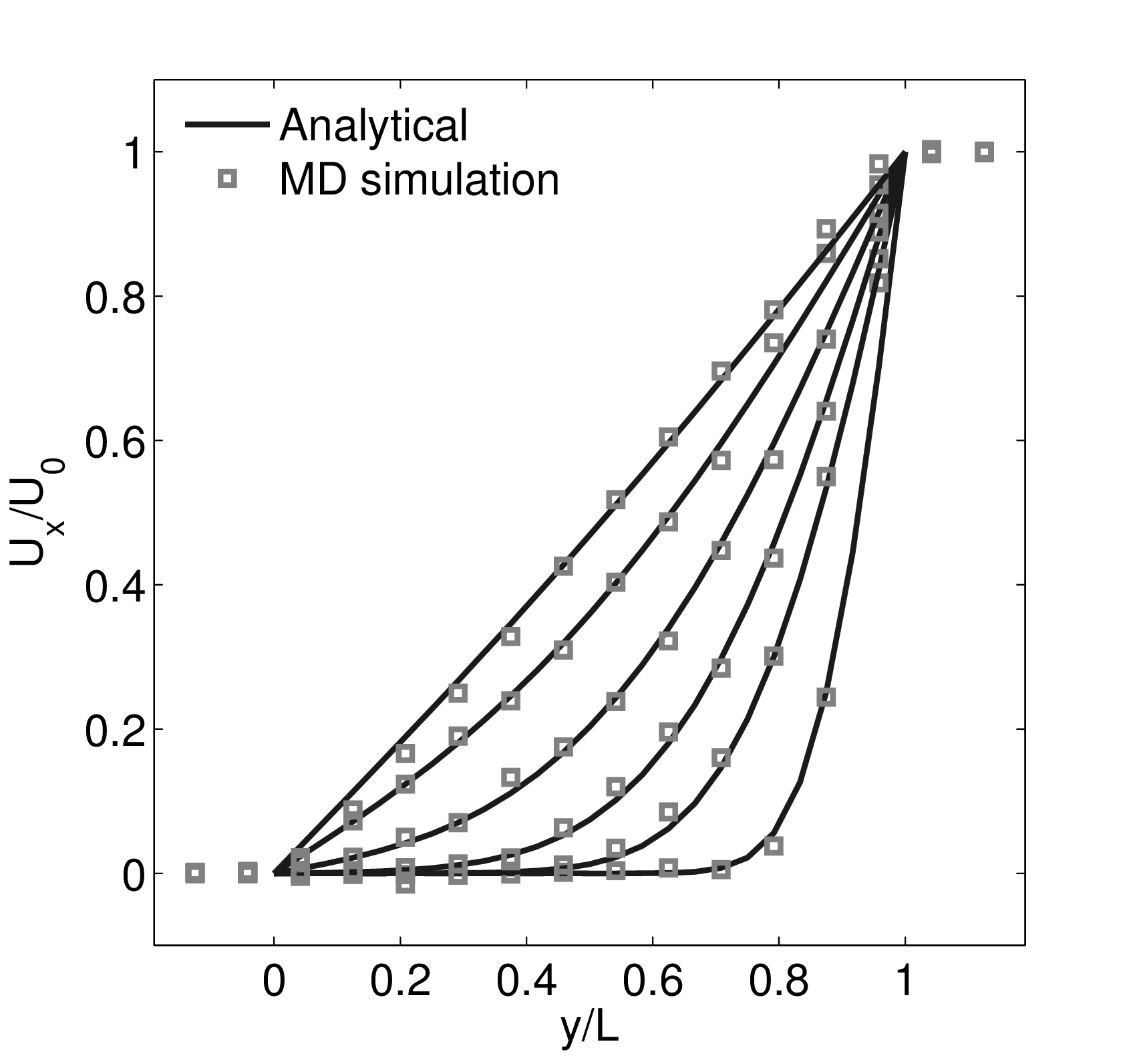
The velocity profile is compared with the analytical solution of the unsteady diffusion equation. Four layers of tethered molecules were used to model each wall, with the top wall given a sliding velocity of, U0 = 1.0 at the start of the simulation, time t = 0. The temperature of both walls was controlled by applying the Nosé-Hoover (NH) thermostat to the wall atoms (Hoover, 1991). The two walls were thermostatted separately, and the equations of motion of the wall atoms were,
![--
r˙i = pi-+ U0n+ , (11a )
mi x
˙pi = Fi + fiext − ξpi, (11b )
( 2 4 )
fiext = ri0 4k4ri0 + 6k6ri0 , (11c)
[∑N -- -- ]
˙ξ = 1-- pn ⋅pn-− 3T0 , (11d )
Qξ n=1 mn](MD_coding56x.png)
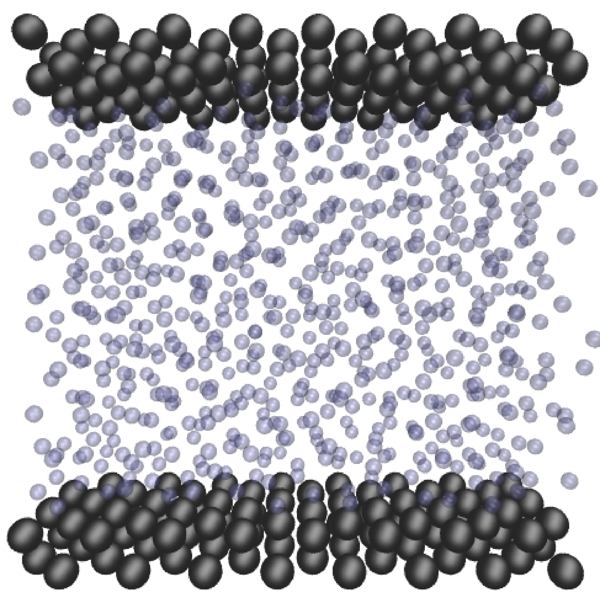
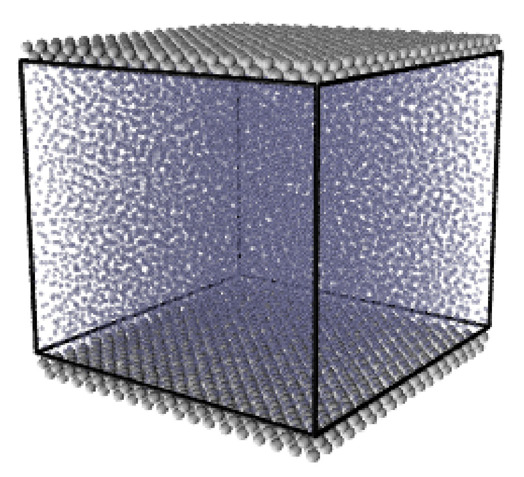
where nx+ is a unit vector in the x− direction (only non-zero for the top wall), mi ≡ m, and fiext is the tethered atom force, obtained using the formula of Petravic & Harrowell (2006) (k4 = 5 × 10³ and k6 = 5 × 10⁶). The vector, ri0 = ri −r0, is the displacement of the tethered atom, i, from its lattice site coordinate, r0. The Nosé-Hoover thermostat dynamical variable is denoted by ξ, T0 = 1.0 is the target temperature of the wall, and the effective time constant or damping coefficient, in Eq. (11d) was given the value, Qξ = NΔt. The simulation was carried out for a cubic domain of sidelength 27.40, of which the fluid region extent was 20.52 in the y−direction (see Figure 14a). Periodic boundaries were used in the streamwise (x) and spanwise (z) directions. The results presented in Figure 14b are the average of eight simulation trajectories starting with a different set of initial atom velocities. The lattice contained 16,384 molecules and was at a density of ρ = 0.8. The molecular simulation domain was sub-divided into 16 averaging slices of height 1.72 and the velocity was determined in each of them. The results show good agreement in both space and time, although some discrepancy is observed near the molecular walls. This is due to molecular layering and stick-slip behaviour near the walls in the molecular system which is not captured in the no-slip boundary assumed in the continuum solution.
The case of Couette flow is revisited repeatedly in this work, using the CFD code and in coupled simulations. This case is chosen because it is simple enough to afford an analytical solution and has been widely studied in the MD, CFD and coupling literature. The Couette flow case for a wide range of pressures has been studied fully, as part of a side project to the work presented herein (Heyes et al., 2012). The setup parameters used in this work are based on this published work Heyes et al. (2012), as are many of the insights into the behaviour of MD and coupled simulations.
3 Continuum code
3.1 Simple Finite Volume Solver
A two dimensional finite volume code which simulates the diffusive terms of the Navier Stokes equation has been developed to test the initial coupling. The unsteady diffusive equations are obtained by simplifying the 3 dimensional Navier Stokes Eq under the assumptions of developed laminar flow, a wide channel in the spanwise direction, negligible pressure gradient and no gravitational effects.
 = =   . . | (12) |
uIJt+1 = u
ijt +  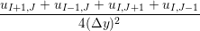 , , | (13) |
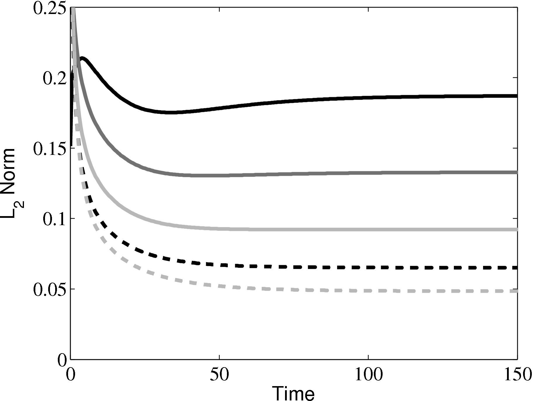
In order to obtain the L2 norm, the square of the discrepancy between analytical and numerical solutions at every point in the domain is obtained. The square root of the sum of these squared discrepencies is the L2 norm. The L2 norm error can be seen to decrease as the solution tends to the steady state and as the number of cells used (resolution) increases in figure 15b. The initial error is attributed to the use of an impulse started plate which the analytical solution would not be able to accurately re-create. The agreement between solutions appears to be good, verifying the CFD code outlined in this section and to be used in coupled Couette flow simulation.
4 Coupling of the DNS and MD algorithms
This section outlines the coupler library. The CPL library website is the most up to date source of information on the software. www.cpl-library.org This validation used version 1.0 of the CPL library code, and the text here is kept for historical records to highlight the validation cases performed during my thesis. Combining the capabilities of the DNS and MD codes requires interfacing and synchronising several elements of the two simulations. Each code models part of the physical problem, and is therefore responsible for a region of the computational domain. An overlap exists between those two domains; MD and continuum information must be “communicated” between the two codes in this region, in order to dynamically couple the two simulations.
Although this method has been demonstrated for a number of small cases, the most significant challenge is to carry out efficient and scalable (thousands of processors) computations of large continuum-molecular coupled systems. Due to its small size, the coupling case in Nie et al. (2004) has been reproduced using the minimal CFD code and the MD solveron a single processor. To move beyond this simple case, a framework must be developed to allow large scale coupling between the two parallel codes.
The proposed framework with separated coupler module and halo exchange is general enough to allow implementation of many of the existing coupling strategies (O’Connell & Thompson, 1995; Nie et al., 2004; Flekkoy et al., 2000; Hadjiconstantinou, 1998; Werder et al., 2005; Delgado-Buscalioni & Coveney, 2003). This generality ensures that the code development will continue to be useful as the field develops.
4.1 Coupler Outline
The coupler (CPL) consists of a series of function calls which are loosely based on the MPI framework in terms of both functionality and scope. They have been developed in FORTRAN 2008 with sufficient generality that they can be used as a language independent API through External functional interfaces. These routines are compiled into a library module which is linked to both the MD and CFD codes. Both codes are then run using the MPI multiple program multiple data paradigm (MPMD) with a call of the form,
mpiexec -n 128 ./md.exe : -n 8 ./cfd.exe.
The codes have entirely separate scopes and can only communicate through the coupler routines. The use of the MPMD framework enforces this separation and prevents conflicts between matching nomenclature in both the MD and CFD codes. It also pre-empts the use of dynamic processor allocation under MPI2, (MPI_spawn), providing a framework to support dynamic load balancing during a simulation.
The coupler consists of three classes of functions – setup, exchange and enquiry. Details of the structure and routines are included below:
- Setup The setup process is run once per simulation and entirely establishes
the relationships between the two codes. The coupler setup routines and all
coupler parameters are contained in a FORTRAN 2003 module
with the protected attribute. This ensures only the three setup
routines located inside this module can changes parameters internal to
the coupler library. This prevents side-effects resulting from the
interface with the CFD/MD codes as well as functions inside the
coupler. The coupler setup functions have extensive error checking to
ensure the inputs are of the correct form and the setup is completed
correctly. A key part of the philosophy of the coupler is that both codes
have copies of an identical set of read-only parameters including
the complete knowledge of the processor topology of both regions.
This ensures inter-communication between the codes is kept to a
minimum.
- CPL_create_comm – Setup MD/CFD INTRA_COMM and INTER_COMM between them. This should be called after both codes have initialised MPI. It defines a global communicator CPL_WORLD_COMM, local intra-communicators MD_COMM/CFD_COMM and an inter-communicator CPL_INTER_COMM between them to allow information exchange between the two domains Gropp et al. (1999b). The COUPLER.in input file is read to define relative processor topologies. The coupler input also includes parameters which are not specified from either of the coupled domains, such as the location and size of the overlap regions, the ratio of timestep between the two codes, as well as the facility to redefine variables in both codes in line with the coupled setup.
- CPL_CFD/MD_init – Input CFD/MD parameters required to setup coupler parameters. Using a minimal set of parameters from both the CFD and MD code, together with the coupler input file, the entire coupling relationship between both domains is setup. The parameters are a minimal set of required and an extended range of optional arguments passed to the CPL_CFD/MD_init function. A hierarchy of communicators are established as part of the mapping process, including communicators containing only topologically overlapping processors CPL_OLAP_COMM and an optimised communicator based on the network topology of the overlapping processors CPL_GRAPH_COMM derived from the MPI_graph function. The details of the communicators are largely hidden from the user as described in the next section.
- Exchange The exchange routines are the core part of the coupler library.
They include the following subroutines:
- CPL_gather – CFD processors gather required data from overlapping MD processors.
- CPL_scatter – CFD processors scatter required data to overlapping MD processors.
- CPL_send – Send from current realm to overlapping processors on other realm.
- CPL_recv – Receive on current realm to overlapping processors on other realm.
All routines require two inputs; an array containing data for all the cells on the calling processor and the global cell numbers specifying the location and range (global extents) of the subset of these cells that the user wants to exchange. The use of global extents prevents the user from requiring any knowledge of the processor’s local numbering system, communicators or the mapping between domains. The global cell number conventions used in exchanges are identical on all processors, so the same input is used on the corresponding exchange routine in the other realm. Only processors with cells in the specified region send and receive the data between the domains. The data array can be of arbitrary size, allowing any number of properties to be exchanged (e.g. density (1), velocity (3) or stresses (9)). As an example, consider sending the MD velocity to be used as the CFD boundary condition for the setup discussed in the background chapter of Smith (2014) thesis. Each MD processor averages the velocity and passes its local array of 3 averaged velocity components per cell to CPL_send. The extents are specified to include all global CFD cells in xz plane at the CFD minimum cell location in y. Every CFD processor posts a corresponding CPL_recv with the same global extents. Every CFD processor on the bottom of the domain then receives an array containing the required boundary cells per processor.
- Enquiry A library of functions to retrieve parameters defined in the other
realm or internal to the coupler. The use of intent out on all enquiry
routines forces the user to make local copies of the returned variables. This
is a further safeguard against corruption of data in the coupler and the
associated side effects.
- CPL_get – Returns any parameter considered protected public in the coupler library.
- CPL_Cart_coords – Returns processor cartesian topology for any processor on either realm.
- CPL_COMM_rank – Returns processor rank in any of the communicators
- CPL_extents – Various extent routines to return cells on
the current processor, in the overlap region or for arbitrary
INPUT=limits subject to the limits of the current processor and
overlap region.
As the coupled topology is set-up at the beginning, all processors have a copy of all processor information in both regions. As a results, the enquiry routines require no communication.
As data from the MD and CFD codes must be manipulated before being passed to the CPL, it is recommended that coupler calls be done in socket routines which contain code written specifically for a given CFD or MD implementation. Calls to the coupler routines in either code can be removed by the use of pre-processing flags or dummy socket routines to allow each code to continue to function separately.
The following flowchart is available in Smith (2014) thesis shows the conceptual operation of a typical coupled setup.
As the coupling module is expected to load balance between both simulations
and interface them efficiently, it is reasonable to expect that the coupled code
will scale as well as the individual codes. The coupling region is local and can
be decomposed spatially for parallel computations in the same manner
as both of the codes it couples. As there is no greater requirement for
communication in the coupling region, the observed scaling should be
similar.
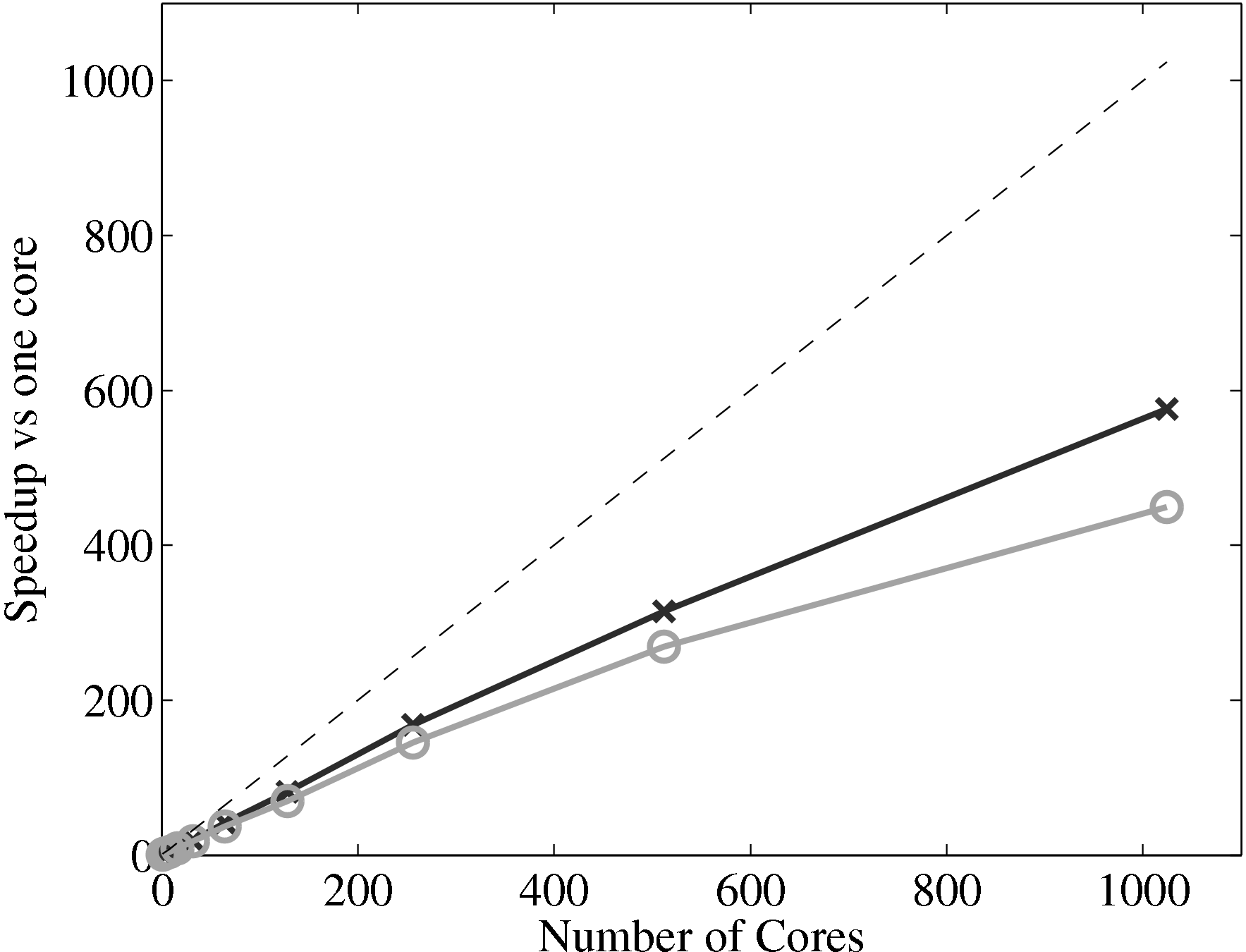
For the case of laminar Couette flow, the computational requirements of the
continuum solver are almost negligible, and the continuum solver is run on a
single processor with 64 cells in x and 7 in y. The speedup of the coupled code
therefore depends almost entirely on the scaling of the MD solver and the
coupler. If the coupler is performing efficiently, this combined speedup can be
expected to be similar to the scaling of the MD solver alone. The scaling of
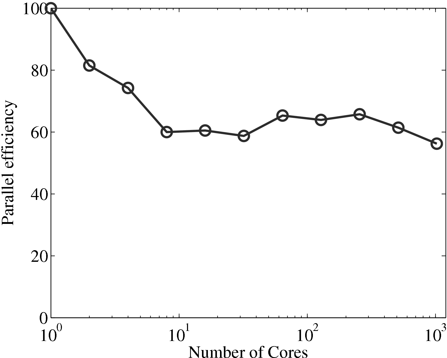
the coupler is compared to the MD solver in Figure 17a, up to 1024
processes. The system size (N = 3,317,760) is the same as used in the
previous all MD scaling tests, section 2.4. The coupled timestep ratio is
50.
Figure 17a demonstrates that the couplers performance only slightly
deteriorates speedup. It is therefore not a severe bottleneck of performance of the
coupled codes.
A part of the development of the coupler library, simple functions
(e.g. sinusoidal profiles) are used to verify the passing is implemented
correctly. A testing suite was written to ‘soak test’ the various coupler
routines for a wide range of processor topologies in both the CFD and MD
domains.
In this subsection, the coupler will be verified using three different types of
coupling scheme from the literature. These include the state coupling of
O’Connell & Thompson (1995) and Nie et al. (2004) both discussed in the state coupling section of
Smith (2014) thesis as well as the flux coupling scheme of Flekkoy et al. (2000) discussed in the flux coupling section (thesis).
A general schematic for the cases in this section is shown in
Figure 18.
The paper by O’Connell & Thompson (1995) presented an investigation of a
sliding bottom wall in the molecular dynamics region with a fixed top wall in the
continuum region. The bottom wall accelerates from stationary with a decaying
exponential velocity of the form uw(t) = U(1 − e−t∕t0) where U = 1 and
t0 = 160 in MD units. The results of O’Connell & Thompson (1995) are
recreated in Figure 19 as part of the coupler verification. These results
are compared to the time evolving analytical solution provided in the
thesis of O’Connell (1995). The essential parameters of the setup are
identical and the reader is referred to O’Connell & Thompson (1995) for full
details. Only the main parameters and differences are summarised here.
The molecular domain had dimensions 11.9 × 18.7 × 8.5 at ρ = 0.81
resulting in N = 1330 molecules. The cutoff length was rc = 2.2 and the
temperature T = 1.1. A bottom wall of thickness 2.34 was kept in place
using the Petravic & Harrowell (2006) tethering potential introduced
in section 2.5.4. The same density was used for the solid walls and the
wall/fluid interaction potential ϵ = 1.0 was chosen instead of the 0.6 used
by O’Connell & Thompson (1995). The domain was terminated by the
O’Connell & Thompson (1995) boundary force applied at the
top to prevent molecules escaping. Application of this boundary force
results in a compression of the MD system causing the propagation of a
shock wave. To prevent this effect, a number of molecules are removed to
ensure the density remains at the intended ρ = 0.81 in the presence of the
boundary force. A Nose-Hoover thermostat was applied instead of the
Langevin thermostat used in O’Connell & Thompson (1995). A number of
thermostatting strategies were tested including z-component only, profile
unbiased thermostat (PUT) and wall only thermostatting. No discernible
difference was found in the behaviour of the profile when compared to the
analytical solution.
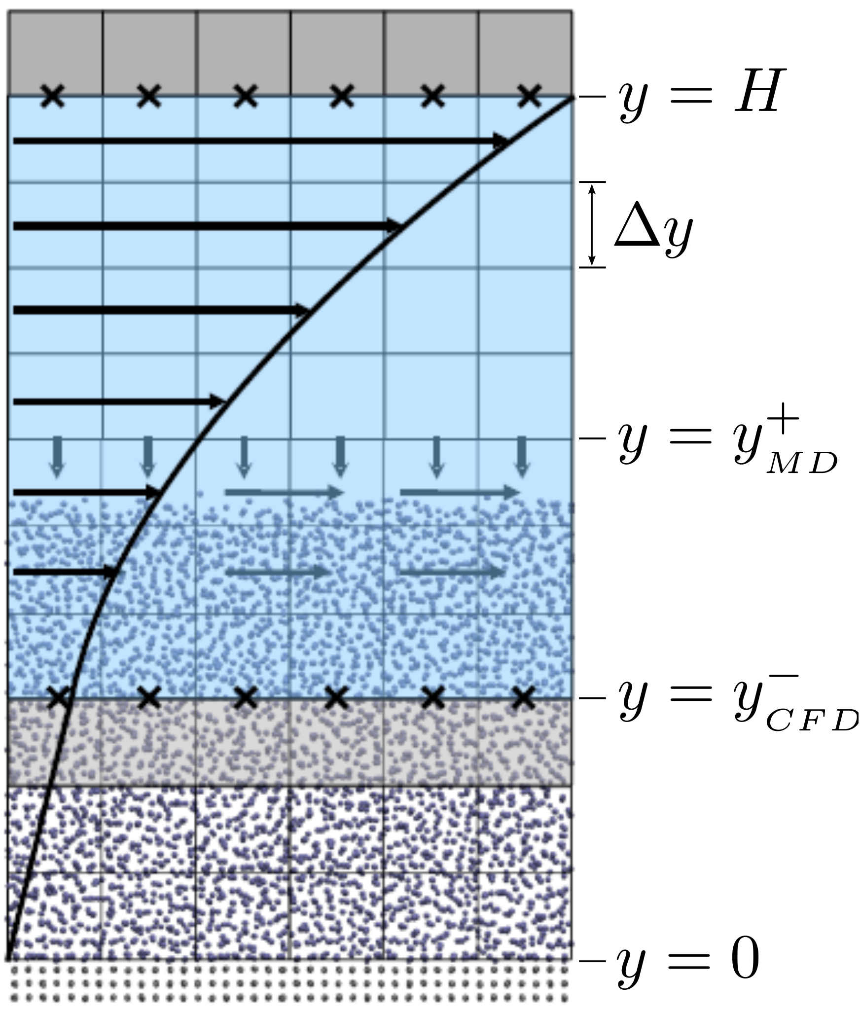
The setup of the coupled case was specified by the various parameters in
Figure 18, including molecular domain top, yMD+ = 18.7, CFD domain
bottom yCFD− = 9.34, total coupled domain height H = 25.68 and cell
size Δy = 2.34. The overlap region consists of four overlap cells. The
arbitrary coupling strength coefficient is set to ξ = 0.01, as in O’Connell &
Thompson (1995).
Molecules in the top MD cell experience the boundary force to
prevent them escaping the domain. In addition, the top cell, together with the
cell below, experiences a constrained force to force the
average molecular velocity inside to match the continuum. The halo cell for the
CFD was obtained by averaging the momentum in the pure
MD region at the location covered by the bottom grey cell in Figure
18.
Please see Smith (2014) thesis4.2 Benchmarking and scalability of the coupled algorithm
 (a) Parallel speedup of the MD solver only (×), coupled code (∘) against the
ideal speedup (−−)
(a) Parallel speedup of the MD solver only (×), coupled code (∘) against the
ideal speedup (−−)
4.3 Verification of the Coupler
4.3.1 O’Connell & Thompson (1995)
The coupling was verified first using the 2D simple finite volume CFD solver outlined in section 3.1 with fixed top boundary condition and bottom boundary passed from the MD region. The CFD solver used a viscosity of μ = 2.14 (or equivalent Reynolds number of Re = 0.378) which was matched to the MD value obtained from Green-Kubo (Green, 1954; Kubo, 1957) calibration calculations.
Good agreement was observed to the analytical solution for an accelerating plate. The setup of this problem applies the moving boundary condition in the molecular region, which in turn drives the continuum due to the coupling between them.
This model implements no mass flux and the scaling parameters ξ is said to cause lagging behind the continuum solution in time evolving flows by Nie et al. (2004). The coupling method presented in the work of Nie et al. (2004) is claimed to ameliorate this problem. The implementation of this method using the CPL library is presented in the next section.
4.3.2 Nie et al. (2004)
This section implements the coupled simulation of Nie et al. (2004). The setup of the coupled simulation in this section aims to be similar to that of the previous section while matching the essential parameters of Nie et al. (2004). As before, the reader is referred to the original work (Nie et al., 2004) for full details of the setup used. The simulation is impulse started Couette flow, where the top wall in the CFD domain was moved at a velocity of uw(t) = 1 and the bottom wall in the molecular region was stationary.
The MD domain size was 34.06 × 34.06 × 34.06 with a density of ρ = 0.81 giving N = 27,200 molecules. The molecular domain was simulated on 4 processes with topology 2 × 2 × 1. The bigger domain size provides better statistics and each cell was twice the size (in each direction) of those used by O’Connell & Thompson (1995). Nie et al. (2004) use the average of 10 MD ensembles, each of width 4.82, to provide boundary conditions for a single CFD instance. The implementation here instead uses a wider domain in z and a single MD simulation. A bottom wall of thickness 2.62 was kept in place using the Petravic & Harrowell (2006) tethering potential introduced in the NEMD section 2.5.4. The same density was used for the solid walls and fluid regions and for simplicity the wall/fluid interaction potential is set to ϵ = 1.0, instead of the 0.6 used by Nie et al. (2004). The cutoff length was rc = 2.2 and the temperature T = 1.1. A Nosè-Hoover thermostat was applied instead of the Langevin. Again application of the thermostat in z only, in a profile unbiased manner or simply thermostatting the wall results in similar agreement to the Couette flow time-evolving analytical solution shown in Figure 20.
The setup of the coupled case was specified by molecular domain top, yMD+ = 31.3, CFD domain bottom yCFD− = 15.6, total coupled domain height H = 52.1 and cell size Δy = 5.12. The overlap was of size 15.6, split into four overlap cells. Molecules in the top MD cell are subjected to the boundary forces to prevent them from escaping. In addition, the top cell, together with the cell below, experiences a constrained forc to ensure average molecular velocties are matched to the continuum. The halo for the CFD was obtained by averaging the pure MD region below the overlap region. The ratio of timesteps between the MD and CFD simulations was 50. Please see Smith (2014) thesis) for details of all forces and averaging methods.
The coupling was verified using the 2D simple finite volume CFD
solver and full 3D DNS code  rans
rans low (run on a single processor).
Both CFD solvers used a viscosity of μ = 2.14 (or equivalent Reynolds
number).
low (run on a single processor).
Both CFD solvers used a viscosity of μ = 2.14 (or equivalent Reynolds
number).
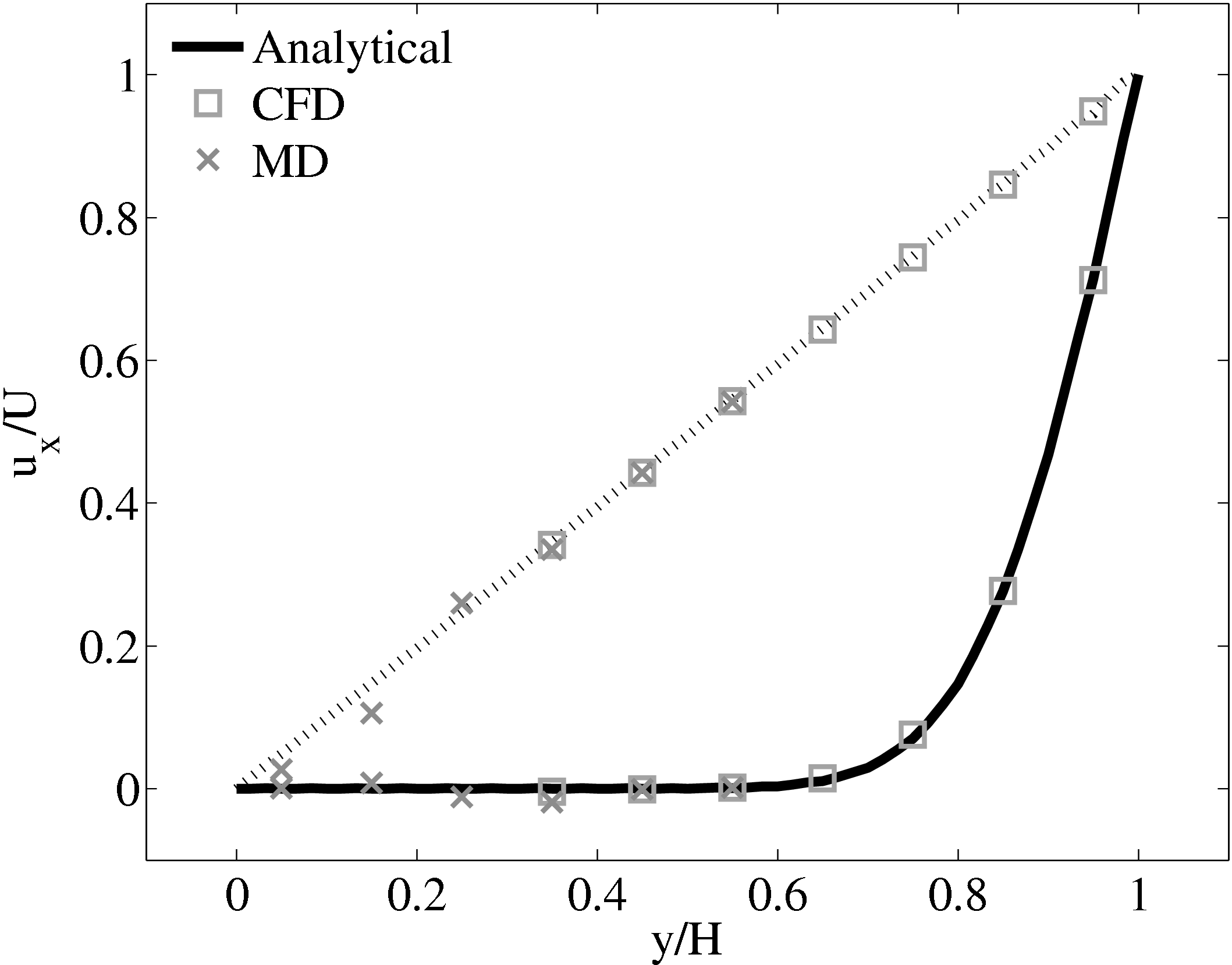
The velocity against time shows good agreement to the analytical solution in Figure 21a.
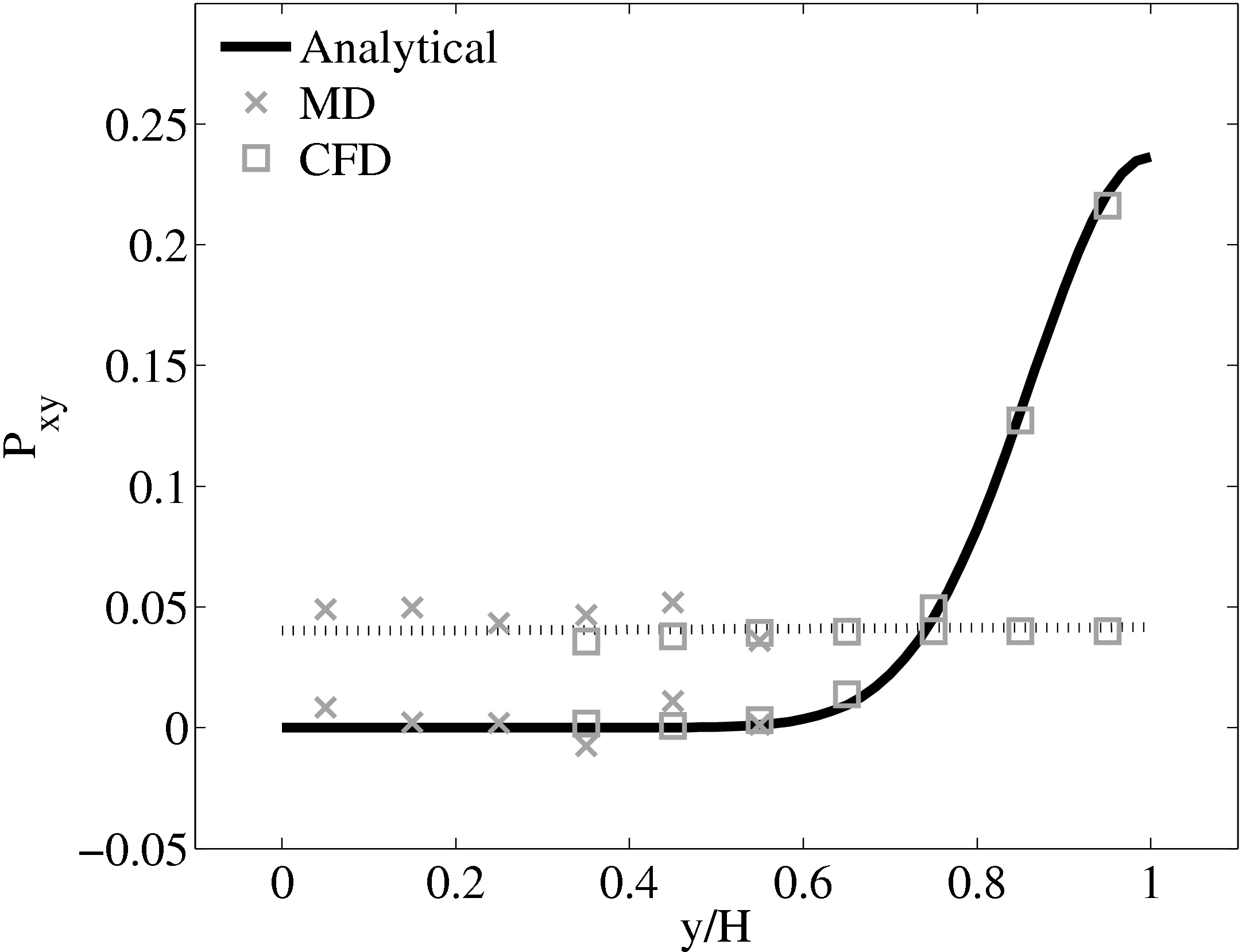
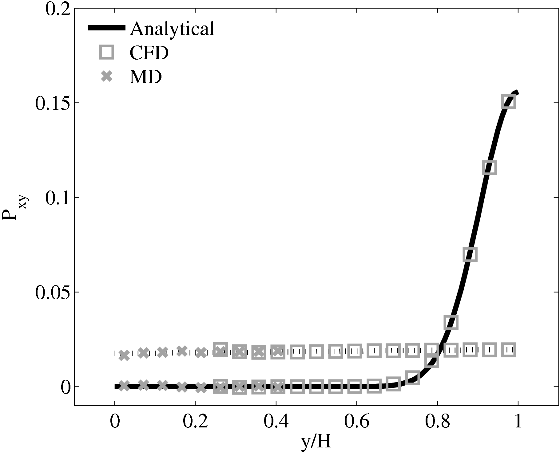
The stress in both the CFD and MD simulation can also be evaluated for the coupled case and the agreement compared to the analytical solution for stress (see appendix thesis). In the MD region, the stress was obtained from the volume average (VA) localisation of the virial stress (Cormier et al., 2001) discussed in the VA section of Smith (2014) thesis. In the CFD region, the stress can be calculated using the hydrodynamic pressure, the gradient of velocity and the shear viscosity. The stress in both simulations and across the coupled region can be seen to match the analytical solution as shown in Figure 21b. The constraint on velocity can be seen to ensure the stress is also matched between both domain. In the next section, the stress itself is constrained, using the flux coupling schemes of Flekkoy et al. (2000).
4.3.3 Flekkoy et al. (2000)
The final verification case is based on the flux coupling work of Flekkoy
et al. (2000). They model Couette flow using an MD domain between two CFD
regions. The results they present are only for steady state Couette flow. This
section extends these results to verify the time evolution of a coupled Couette
flow with flux coupling. A much larger molecular domain was used to test the
coupler for large system sizes. This also addresses the higher averaging
requirement of flux coupling outlined in statistical error section of Smith (2014) thesis. The MD domain size was
164.2 × 51.3 × 41.0 at density ρ = 0.8, resulting in N = 276,480 molecules. The
molecular domain was simulated on 32 processes with topology 8 × 2 × 2. The
bottom wall was tethered with a thickness of 5.13 and a Nosé-Hoover
thermostat was applied to only the wall molecules with a temperature setpoint
of T = 1.0. The WCA potential was used (rc = 2 ) for computational
efficiency.
) for computational
efficiency.
The paper by Flekkoy et al. (2000) is unclear of exact domain sizes but states that cells of size 7.6 are employed with 10 cells shown in the MD domain on their Fig. 2 (i.e. an MD domain of 76.0). This MD region is sandwiched between two CFD domains in Flekkoy et al. (2000) with a coupling region on each side of width 22.8. Only one sided coupling was used here, again based on the setup shown in Figure 18. A domain of similar height without the bottom coupling region was used – yMD+ = 46.17. The cells were chosen to be slightly smaller than Flekkoy et al. (2000) and consistent with Nie et al. (2004) at Δy = 5.13. The continuum domain bottom was located at yCFD− = 25.65 and the total domain was twice the size of Nie et al. (2004) with a height of H = 107.8
The constraint force of Flekkoy et al. (2000) with weighting function given in Smith (2014) thesis) applied both the appropriate direct pressure and shear pressure to the MD domain. As the pressure applied is not designed to prevent molecules from escaping, only to match the continuum pressure, specular walls are also employed. These reflect molecules back with identical x and z velocities and exactly opposite y components of velocity. Specular walls are chosen as the continuum solver was incompressible and does not expect a mass flow into the bottom of the continuum domain, therefore restricting mass flux is consistent. Moving these walls with a mean velocity, as in the work of (Werder et al., 2005), was unnecessary as the mean flow rate in the wall normal direction is, on average, zero for this case.
The viscosities are also matched in this simulation with continuum viscosity
set to μ = 1.6 (again from Green-Kubo autocorrelation functions). The
coupling was between the MD and the full 3D DNS code ranslow
with Reynolds number Re = 0.5. The parallel nature of the DNS code
was employed with the 32 × 16 × 8 CFD cells split between 4 × 2 × 1
processes.
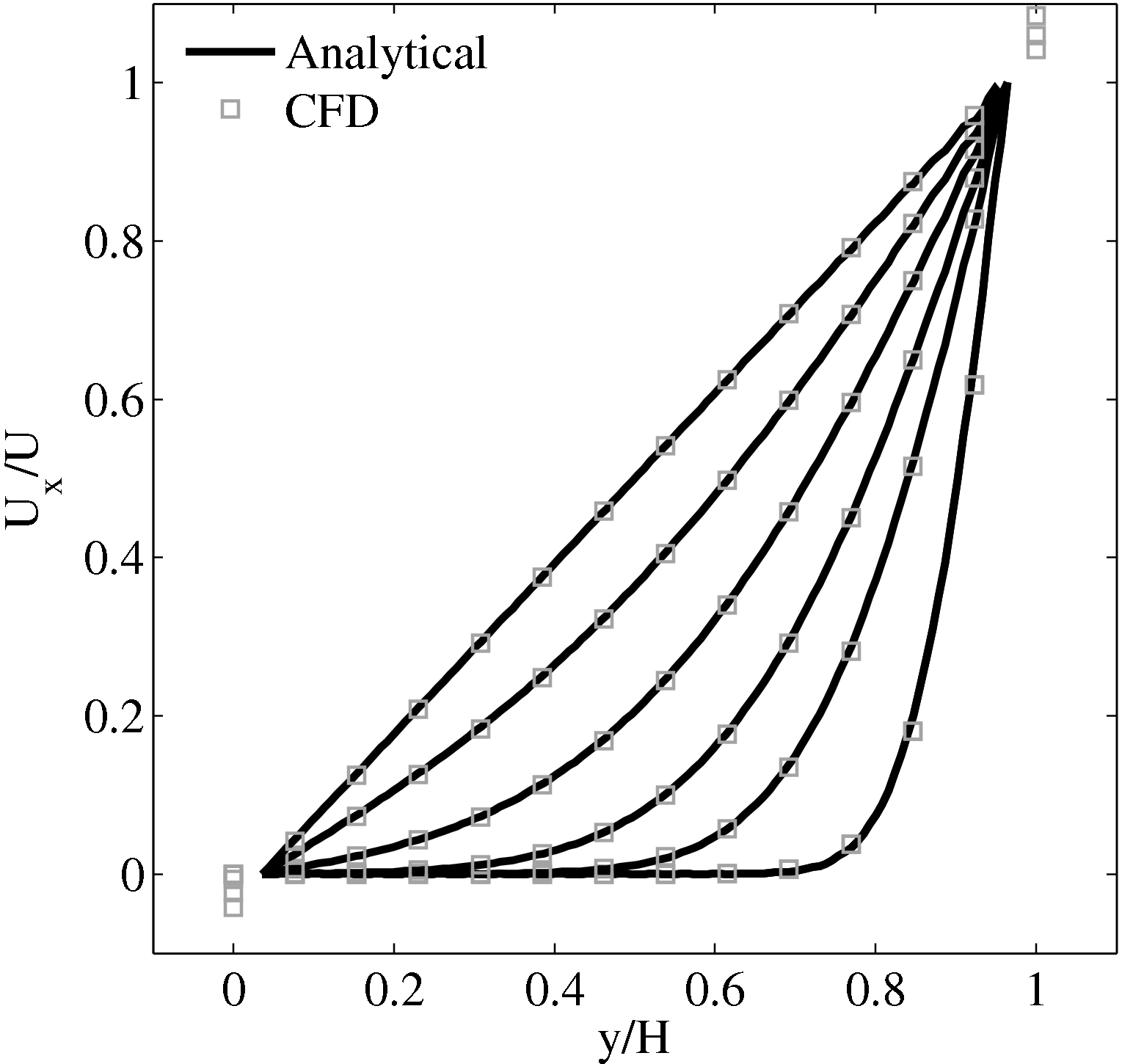
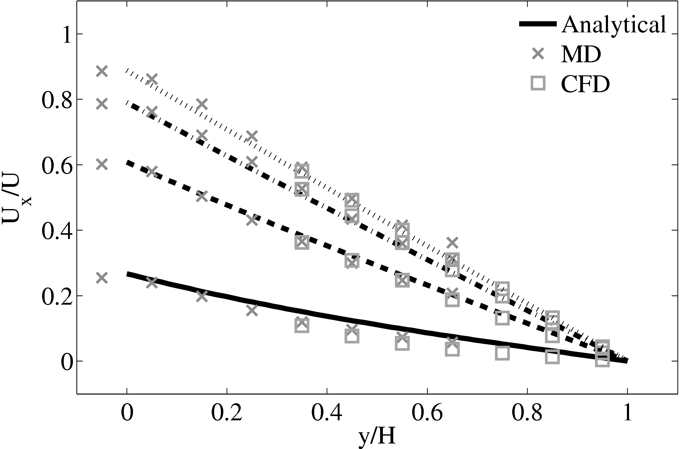
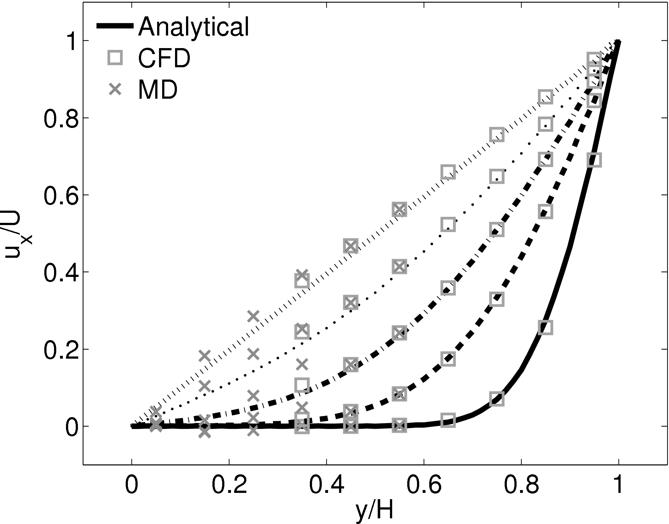
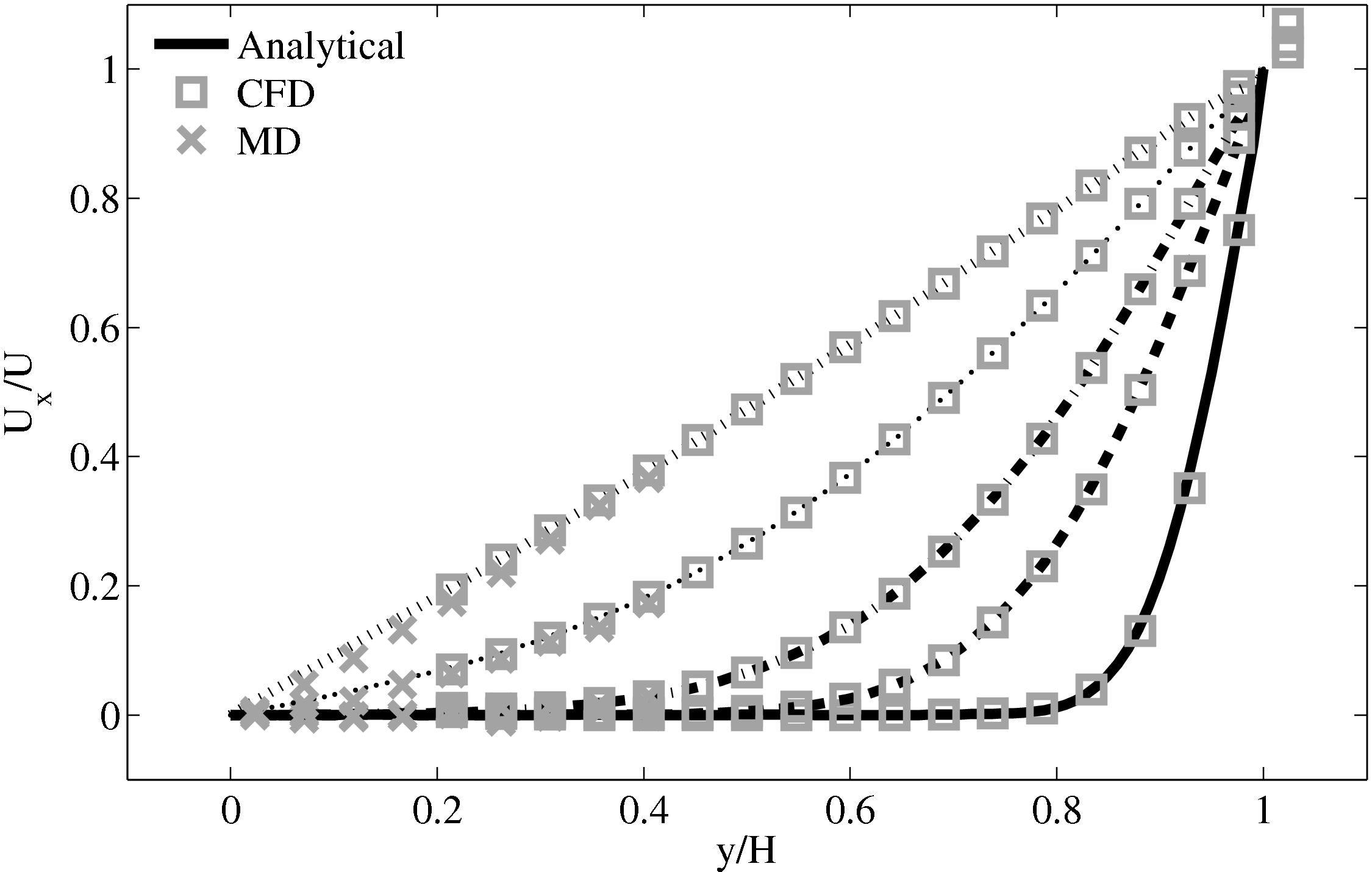
The coupled solution for velocity is compared to the analtical solution in Figure 22. Good agreement is observed at equivalent times to those shown for Nie et al. (2004) in the previous section. As the domain is over 3 times the size of the previous Nie et al. (2004) case, the time scales are proportional to the square of the domain height and are scaled accordingly. Note the greater number of symbolds due to the much greater numbers of cells in both domains.
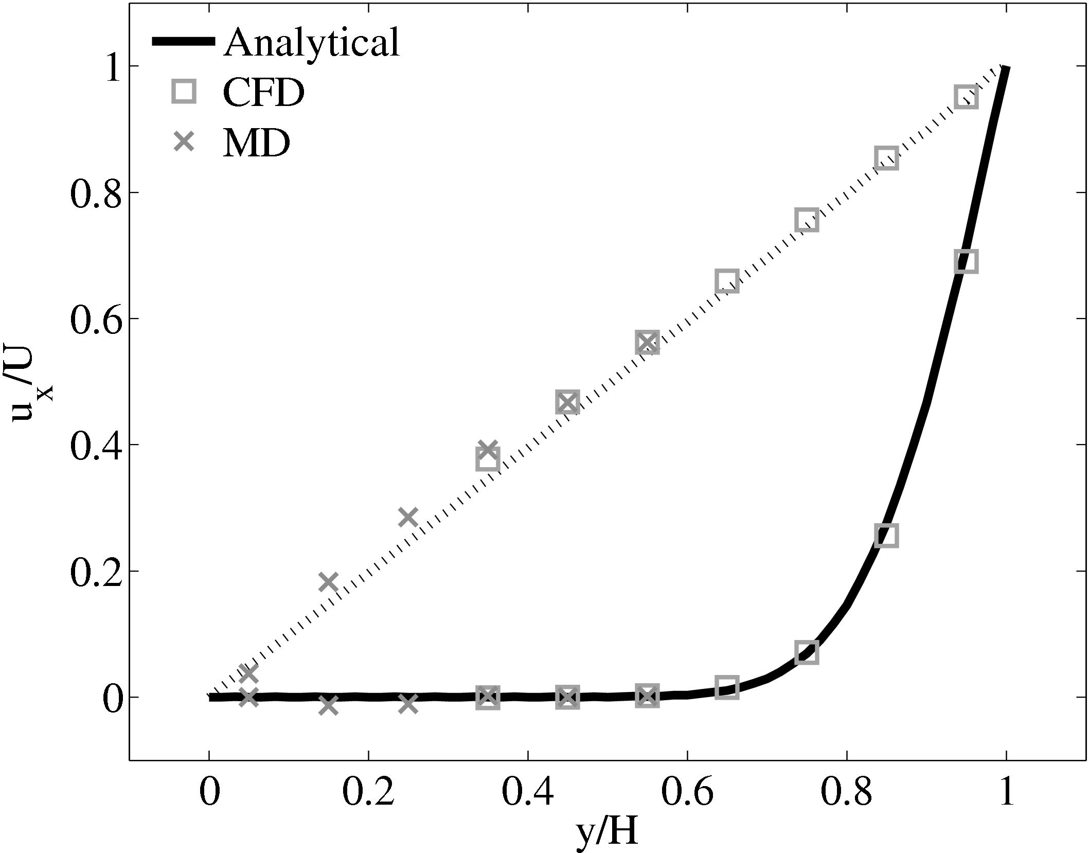
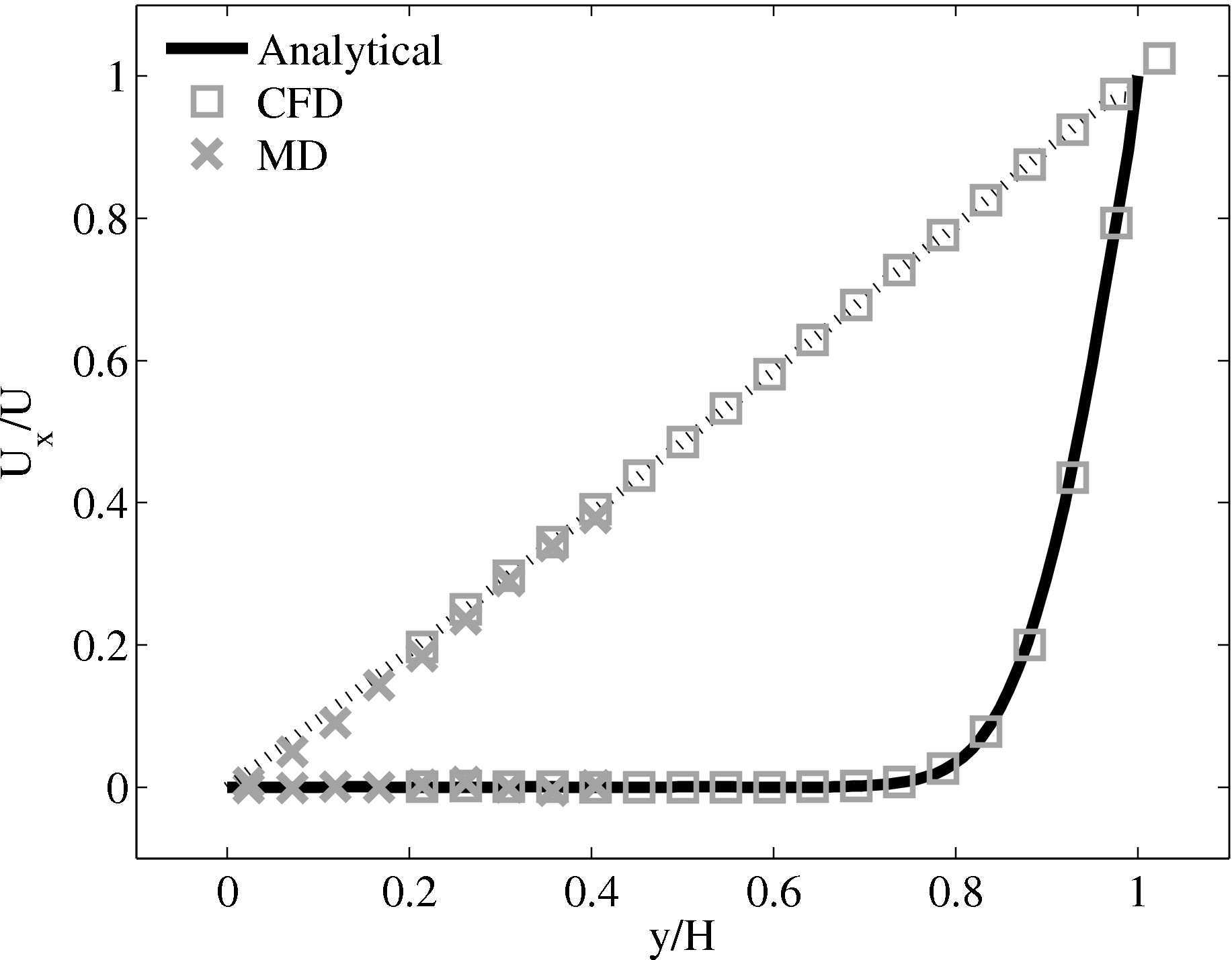
As the stress in both regions was matched by the coupler, this is seen to match in Figure 23b. The velocity can also be seen to agrees in Figure 23a as a result of this stress matching scheme. The near wall agreement in Figure 23a appears to be superior to the Nie et al. (2004) coupling shown in Figure 21a. This is a consequence of the larger system size which reduces the effect of near wall molecular behaviour and improves velocity averages.
The halo for the CFD (bottom grey cells in Figure 18) was obtained by averaging the momentum in the pure MD domain below the overlap region in line. This is a departure from the work of Flekkoy et al. (2000) who average the stresses from the MD region. The manner in which to obtain the stress tensor from the MD is not clear (as discussed in section flux pressure in Smith E (2014) thesis. This mixed coupling is based on the work of Ren (2007), where flux-state coupling is found to be stable, while flux-flux coupling was found to be unstable. There are also concerns about the sample requirements, which are said to be prohibitive for flux schemes in Hadjiconstantinou et al. (2003). However, a parameter study of error in appendix of (thesis) which demonstrate these averages requirements for flux shemes, while often large, are not prohibitive for all cases. Despite this, the mixed flux-state exchange was deemed to be a simpler and more robust way to test the coupling software.
Having verified the coupler gives identical results using both flux and state coupling, the impact of specifying the wrong viscosity is evaluated in the next section. The agreement of state based coupling schemes is shown to be contingent on a consistent viscosity being specified in both domains. The impact of this finding is then discussed.
4.4 Mismatched Viscosity in Couette Flow
The case of coupled Couette flow with a mismatch of viscosity between the continuum and molecular systems is considered in this subsection.
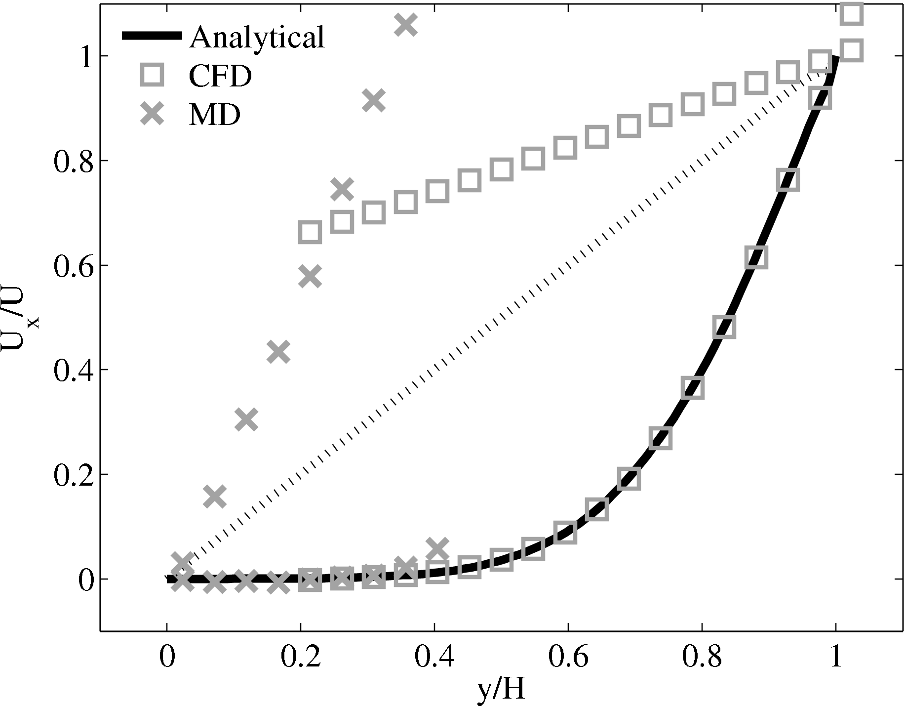
When coupling the continuum and molecular systems, the scaling between the two regions must be consistent. As discussed in class="cmbx-10x-x-109">(thesis) the continuum and molecular domains are scaled based on different parameters. The molecular region is based on length scale ℓ, mass m and energy ϵ, while the continuum is dependent on the Reynolds number Re = ρUL∕μ. The two regions are matched by ensuring the length scales ℓ vs. L and densities ρCFD vs. ρMD = ρMD(m,ℓ) are consistent. The velocity or stress matching is then ensured by the coupling mechanism. Viscosity is a tuneable parameter in the continuum but it is a measureable quantity in a molecular simulation, not an input parameter. Nie et al. (2004) use a viscosity of μ = 2.14 based on previous simulations. As shown in the previous subsection, using this pre-matching of viscosity, good agreement is observed for both the velocity and stress between both systems, Figure 21. For the case where the viscosities are not the same in both regions, the velocity profiles can be seen to match but the stresses do not, Figure 24.
 (a) Mis-matched viscosity μCFD = 10.0, μMD =
2.14
(a) Mis-matched viscosity μCFD = 10.0, μMD =
2.14 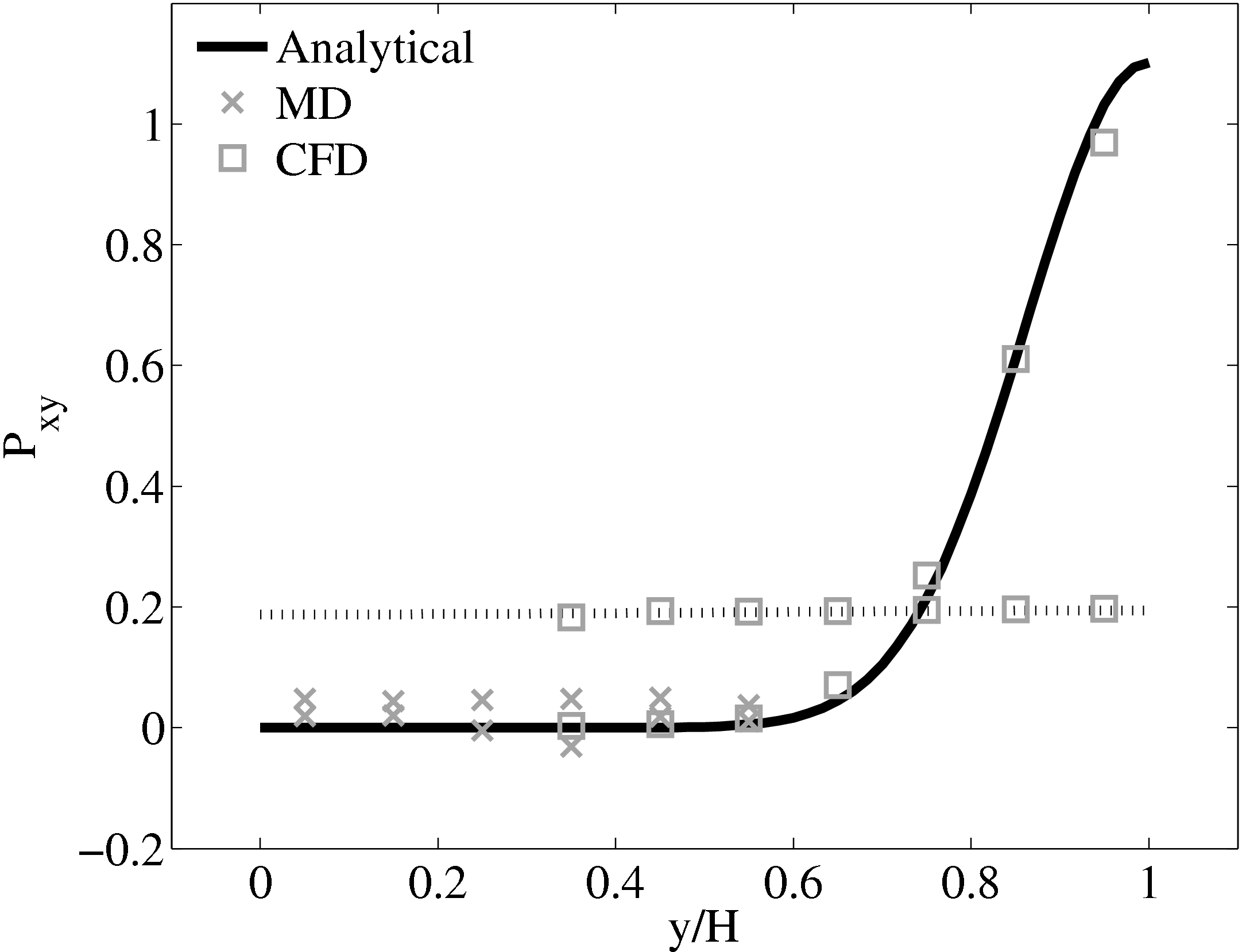 (b) Mis-matched viscosity μCFD = 10.0, μMD =
2.14
(b) Mis-matched viscosity μCFD = 10.0, μMD =
2.14
Consider next the flux couping of Flekkoy et al. (2000). The use of the same viscosity in both domain (μ = 1.6) obtained by prior simulation, Figure 23 in the previous subsection showed good agreement for both velocity and stresses. The use of different viscosity in both regions results in disagreement in the velocity but good agreement in the stresses, Figure 25.
 (a) Mis-matched viscosity μCFD = 10.0, μMD =
2.14
(a) Mis-matched viscosity μCFD = 10.0, μMD =
2.14 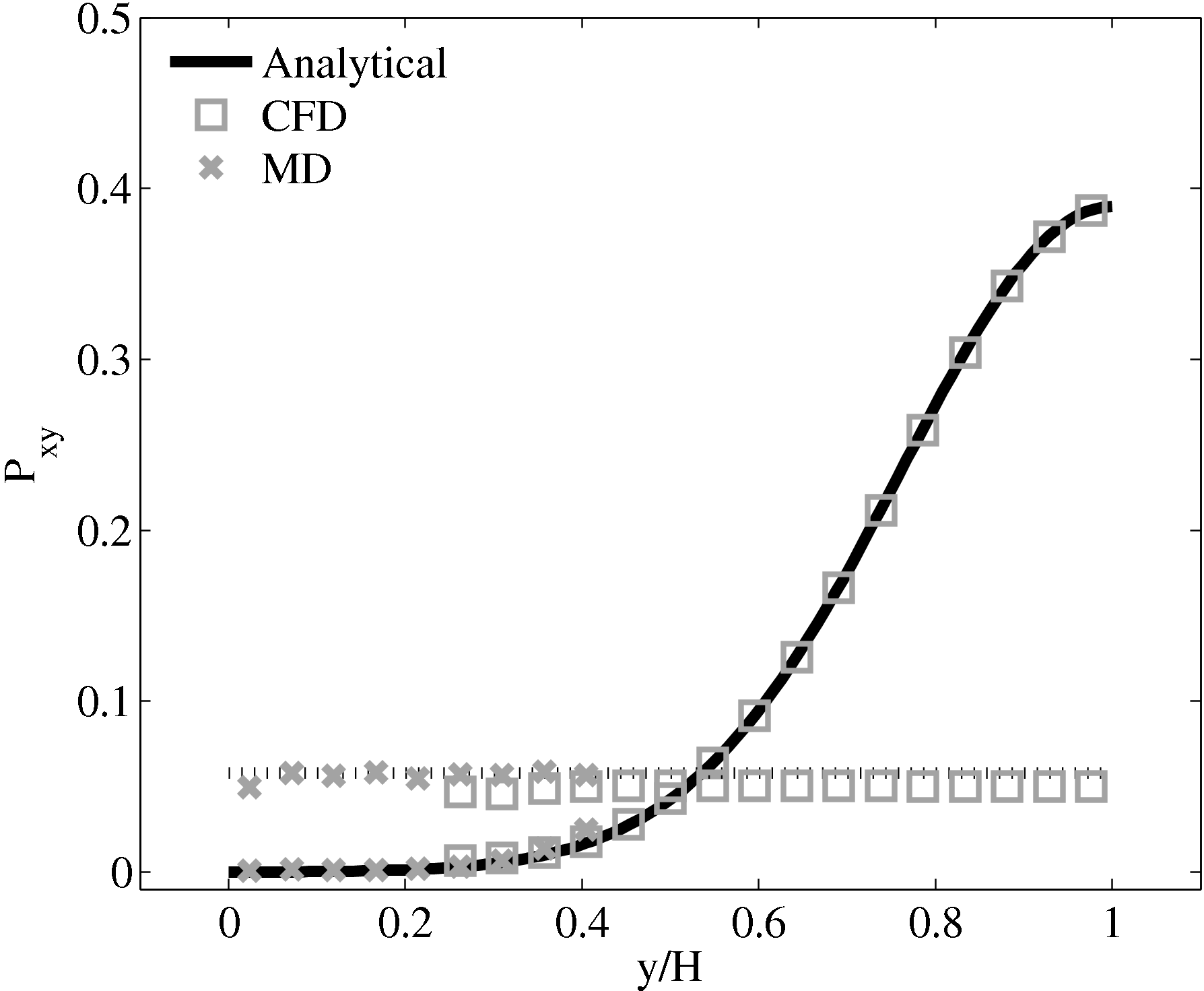 (b) Mis-matched viscosity μCFD = 10.0,
μMD = 1.6
(b) Mis-matched viscosity μCFD = 10.0,
μMD = 1.6
The results for a mismatched stress in figure 25 are consistent with the simulation of two phase fluids with different viscosities. Molecular fluid will typically experience different viscosity measurements in the vicinity of the walls or at high shear rates (shear thinning). By using state coupling, this behaviour would not be correctly transmitted to the CFD realm as a constant viscosity is implicitly assumed throughout the MD. In addition, it is possible to unknowingly simulate cases with viscosity difference and still obtain apparently correct velocity profiles. The conclusion is that the flux coupling scheme are more general as they require no assumption of the viscosity in the MD region, as they simply apply a force consistent with the current state of stress in the CFD.
The results from this study of mismatched viscosity suggest that a more stringent set of tests are required in order to establish the consistency between the two realms of a coupled simulation, a problem that motivates the next page with the development of a consistent control volume framework for both systems. In addition, flux coupling scheme are more general and should be preferred in the computational implementation of a general purpose coupling simulation tool, which was the aim of this section. As they are not currently derived from a constrained dynamics approach, some theoretical development is required and this motivates the work on control volumes (thesis).
This section has introduced a coupling library for simulation of large scale case on many processors. The intention was to couple simulations which approach scales of engineering interest, including the modelling of turbulent phenomenon. However, there are a number of problems to overcome before a generalised coupling scheme can be implemented.
5 Overview
This section includes the details of the software developments and verifications in the development of a coupled continuum-molecular solver. In order to couple molecular dynamics (MD) to continuum computational fluid mechanics (CFD), a new MD code was developed, a CFD code was adapted and a coupling library designed to manage the data exchange between them.
In section 2, the details of the development and testing of a new MD code were presented. The MD code was designed to use cell/neighbour lists, Hilbert curve re-ordering and other optimisations to obtain similar serial speeds to LAMMPS. The code is then parallelised using MPI to allow running on high performance computing platforms. The parallel performance is tested and shows 94% efficiency when scaling from 8 processors to 1024. The MD code was verified by checking the energy conservation, trajectory agreement (and divergence), radial distribution function, phase diagrams and simulation of Couette flow. The optimised MD code is therefore ready for large-scale simulation of molecular dynamics and coupling problems.
Section, 3, outlined the development and verification of a simple CFD code. This was used as part of the development of the coupling library and for simple CFD test cases.
The final part of this page, section 4, outlined the development of a robust and minimal coupling (CPL) library. This was designed as a language independent APIs using FORTRAN 2008, which implements the data exchange between the CFD and MD codes. Implementation of coupling should be as simple as initialising the CPL module by passing the key simulation parameters from both MD/CFD codes. The data can be exchanged by CPL_send/CPL_recv calls which ensure all data is passed correctly. The library was soak tested and verified for range of cases and topologies from the literature (O’Connell & Thompson, 1995; Nie et al., 2004; Flekkoy et al., 2000). In order to test the scaling of the coupler, performance of a CPL simulation was compared to an uncoupled case. The difference in speedup on 1024 processor was found to be 575 for the full MD and 449 for a coupled case, compared to the ideal 1024. The coupler is therefore seen to have minimal impact on the scaling of the two codes.
References
Allen, M. P. & Tildesley, D. J. 1987 Computer Simulation of Liquids, 1st edn. Clarendon Press, Oxford.
Anderson, J. A., Lorenz, C. D. & Travesset, A. 2008 General purpose molecular dynamics simulation fully implemented on graphical processing units. J. of Comp. Phys. 227, 5342.
Anton, L. & Smith, E. 2012 Scalable coupling of molecular dynamics (md) and direct numerical simulation (dns) of multi-scale flows. Tech. Rep..
Brown, W. M., Wang, P., Plimpton, S. J. & Tharrington, A. N. 2011 Implementing molecular dynamics on hybrid high performance computers-short range forces. Comp. Phys. Comms. 182, 898.
Cormier, J., Rickman, J. M. & Delph, T. J. 2001 Stress calculation in atomistic simulations of perfect and imperfect solids. J. Appl. Phys 89, 99.
Delgado-Buscalioni, R. & Coveney, P. 2003 Continuum-particle hybrid coupling for mass, momentum, and energy transfers in unsteady fluid flow. Phys. Rev. E 67, 046704.
Evans, D. J. & Morriss, G. P. 2007 Statistical Mechanics of Non-Equilibrium Liquids, 2nd edn. Australian National University Press, Canberra.
Flekkèy, E. G., Wagner, G. & Feder, J. 2000 Hybrid model for combined particle and continuum dynamics. Europhys. Lett. 52, 271.
Green, M. S. 1954 Markoff random processes and the statistical mechanics of time-dependent phenomena. ii. irreversible processes in fluids. The Journal of Chemical Physics 22 (3), 398–413.
Gropp, W. D., Lusk, E. L. & Skjellum, A. 1999a Using MPI: Portable Parallel Programming With the Message-Passing Interface, Volume 1, 1st edn. MIT Press.
Gropp, W. D., Lusk, E. L. & Thakur, R. 1999b Using MPI-2:Advanced Features of the Message-Passing Interface, Volume 2, 1st edn. Falcon.
Hadjiconstantinou, N. G. 1998 Hybrid atomisticcontinuum formulations and the moving contact-line problem. PhD thesis, MIT(U.S.).
Hadjiconstantinou, N. G., Garcia, A. L., Bazant, M. Z. & He, G. 2003 Statistical error in particle simulations of hydrodynamic phenomena. J. Comp. Phys. 187, 274.
Heyes, D. M., Smith, E. R., Dini, D., Spikes, H. A. & Zaki, T. A. 2012 Pressure dependence of confined liquid behavior subjected to boundary-driven shear. J. Chem. Phys 136, 134705.
Hirsch, C. 2007 Numerical Computation of Internal and External Flows, 2nd edn. Elsevier, Oxford.
Hoover, W. G. 1991 Computational Statistical Mechanics, 1st edn. Elsevier Science, Oxford.
Humphrey, W., Dalke, A. & Schulten, K. 1996 Vmd - visual molecular dynamics. J. Molec. Grap. 14.1, 33.
Itterbeek, V. & Verbeke, O. 1960 Density of liquid nitrogen and argon as a function of pressure and temperature. Physica 931 (26).
Kubo, R. 1957 Statistical-mechanical theory of irreversible processes. i. general theory and simple applications to magnetic and conduction problems. Journal of the Physical Society of Japan 12 (6), 570–586.
Lutsko, J. F. 1988 Stress and elastic constants in anisotropic solids: Molecular dynamics techniques. J. Appl. Phys 64, 1152.
Nethercote, N. 2004 Dynamic binary analysis and instrumentation. PhD thesis, University of Cambridge.
Nie, X. B., Chen, S., E, W. N. & Robbins, M. 2004 A continuum and molecular dynamics hybrid method for micro- and nano-fluid flow. J. of Fluid Mech. 500, 55.
NIST 2013 Benchmark results for the lennard-jones fluid.
NVIDIA 2010 NVIDIA CUDA C Programming Guide, 3rd edn. NVIDIA Corporation, 2701 San Tomas Expressway, Santa Clara, CA 95050.
O’Connell, S. 1995 The development of a molecular dynamics - continuum hybrid computation for modeling fluid flows. PhD thesis, Duke University (U.S.).
O’Connell, S. T. & Thompson, P. A. 1995 Molecular dynamics-continuum hybrid computations: A tool for studying complex fluid flow. Phys. Rev. E 52, R5792.
Petravic, J. & Harrowell, P. 2006 The boundary fluctuation theory of transport coefficients in the linear-response limit. J. Chem. Phys. 124, 014103.
Plimpton, S. 1995 Fast parallel algorithms for short range molecular dynamics. J. of Comp. Phys. 117, 1.
Plimpton, S., Crozier, P. & Thompson, A. 2003 LAMMPS Users Manual - Largescale Atomic/Molecular Massively Parallel Simulator, 7th edn. http://lammps.sandia.gov.
Rapaport, D. C. 2004 The Art of Molecular Dynamics Simulation, 2nd edn. Cambridge University Press, Cambridge.
Ren, W. 2007 Analytical and numerical study of coupled atomistic-continuum methods for fluids. J. of Comp. Phys. 227, 1353.
Shende, S. & Malony, A. D. 2006 The tau parallel performance system. Int. J. High Perf. Comp. Apps. 20, 287.
Smith, E., Trevelyan, D. & Zaki, T. A. 2013 Scalable coupling of molecular dynamics (md) and direct numerical simulation (dns) of multi-scale flowspart 2. Tech. Rep..
Smith, E. R., Heyes, D. M., Dini, D. & Zaki, T. A. 2012 Control-volume representation of molecular dynamics. Phys. Rev. E. 85, 056705.
Smith, E. R. & Trevelyan, D. 2013 Cpl-library.
Spoel, D. V. D., Lindahl, E., Hess, B., Groenhoff, G., Mark, A. E. & Berendsen, H. J. C. 2005 Gromacs: Fast, flexible, and free. J. of Comp. Chem. 26, 1701.
Werder, T., Walther, J. H. & Koumoutsakos, P. 2005 Hybrid atomistic continuum method for the simulation of dense fluid flows. J. of Comp. Phys. 205, 373.
Yamell, J. L., Katz, M. J., Wenzel, R. G. & Koenig, S. H. 1973 Structure factor and radial distribution function for liquid argon at 85k. Phys. Rev. A 7, 2130.